• Profile
• Physics
• Programming
• Tutorial
• More
  • link 1
  • link 2
  • link 3

Part 1: Select the Primary beam and fragment

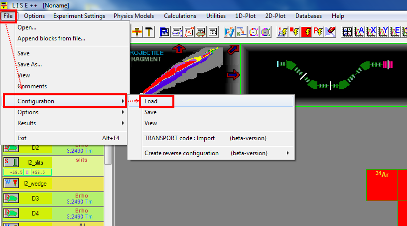
Before staring any calculation, we should use the latest configuration.
menu bar --> File --> Configurations --> Load.
Here we select MSU --> A1900_2015.lcn

Primary beam

Go to http://nscl.msu.edu/users/beams.html, to see what the primary beam options we have.

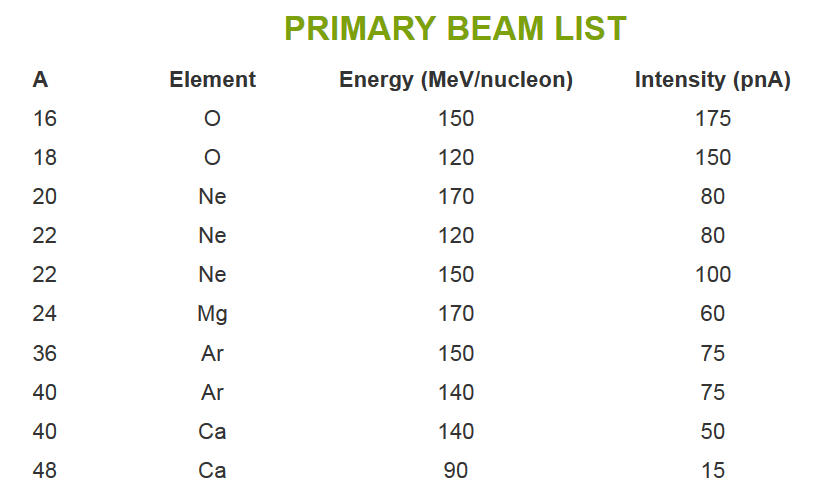
If we would like to have $^{22}$Al as our secondary beam, it has 13 protons and 9 protons.
Let's try to use $^{36}$Ar as our primary beam, which has 18 protons and 18 neurons.
When $^{36}$Ar hits $^{9}$Be, we can create the $^{22}$Al fragment, along with many other nuclei as contaminations.
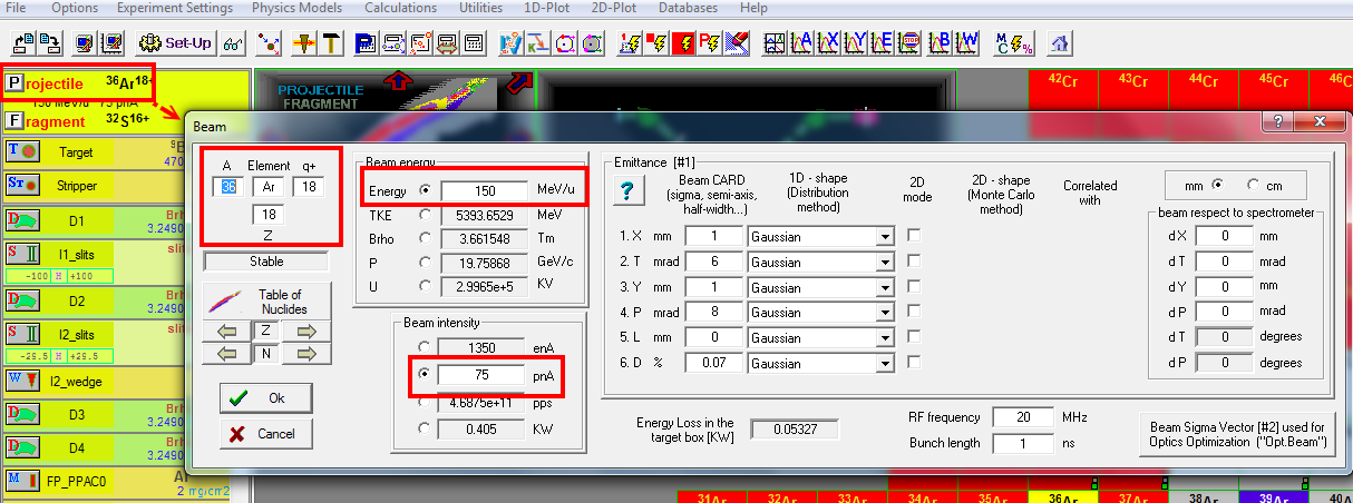
As listed above for the $^{36}$Ar beam, we will have 150 MeV/u as beam energy and 75 pnA for beam intensity.

We input the $^{36}$Ar beam information into LISE.

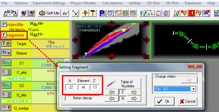
Then setup the fragment as $^{22}$Al.

We have calculate the $^{9}$Be optimal thickness for producing $^{22}$Al when using $^{36}$Ar as the primary beam.
(how many $^{22}$Al ions will be created and pass through the $^{9}$Be)
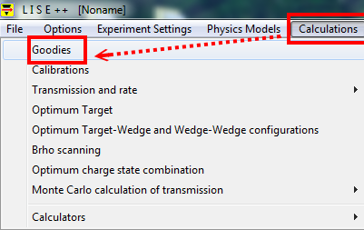
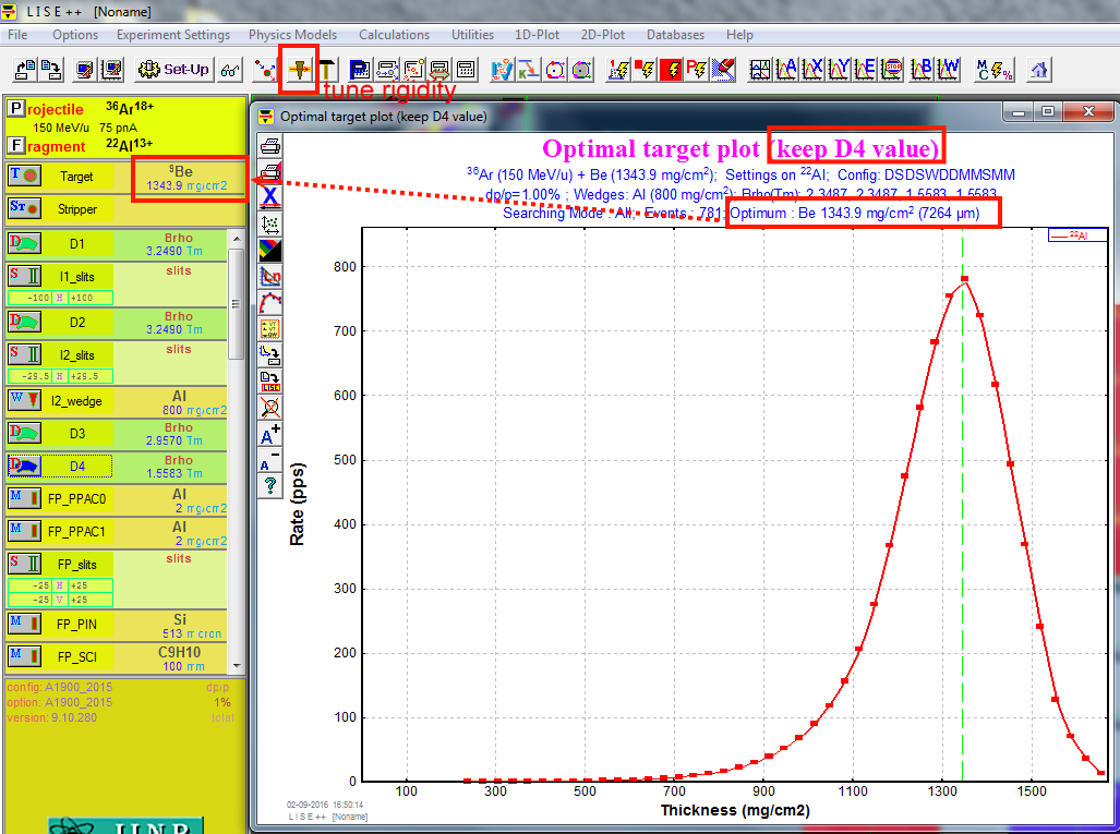
At the menu bar --> "Calculations" --> "Optimum Target"



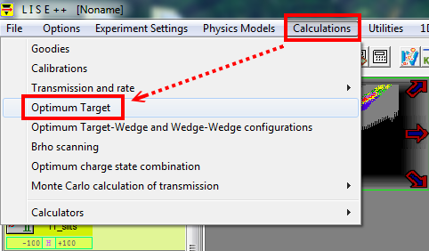
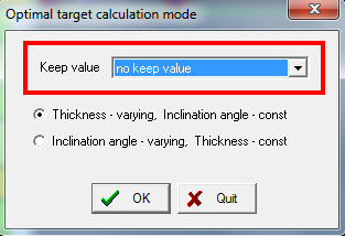
I use the default options "no keep value".
Personal note: "keep value D4"



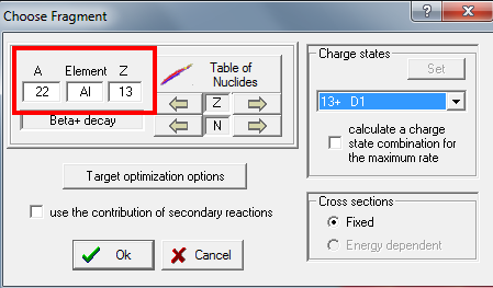
key in the $^{22}$Al information again.



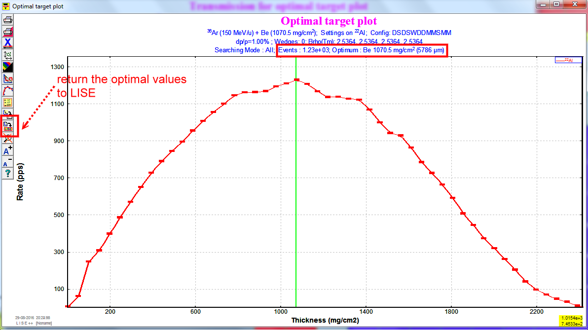
We will see a plot with x axis is the thickness any y axis is the rate
The optimal thickness is 1070.5 $mg/cm^{2}$, and we have $1.23 \times 10^{3}$ for the $^{22}$Al ions.
Next, we return the optimal thickness value to LISE, just click the icon on the left.

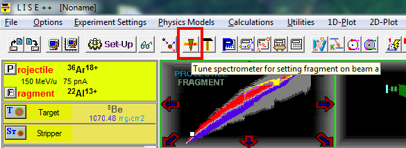
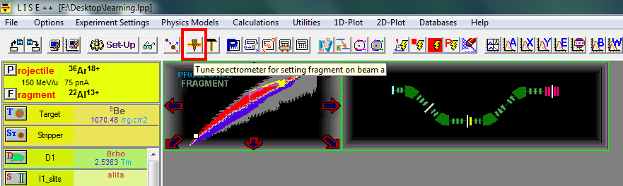
Part 2: Spectrometer setting

After setting up the primary beam, fragment, the $^{9}$Be thickness, then we should tune the spectrometer.
Just click the following button, and we will use this button several times.



At the left hand side, there is a panel show the parameters of the spectrometer. By default configuration of A1900 spectrometer, the Aluminum wedge thickness is zero. It results in magnetic rigidity $B_{\rho}$ for dipole magnet D1, D2, D3, and D4 is the same.

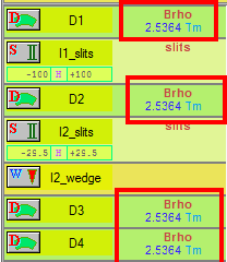
Note: $B_{\rho}$ = = $\frac{momentum}{charge}$, a quantity to describe how stiff when we want to turn the beam.


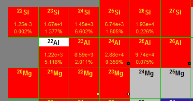
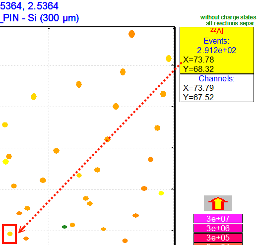
For observing the yield (total events) and the transmission efficiency in %,
use the mouse to double right click the nuclei in the chart.

part 3 : Momentum acceptance setting

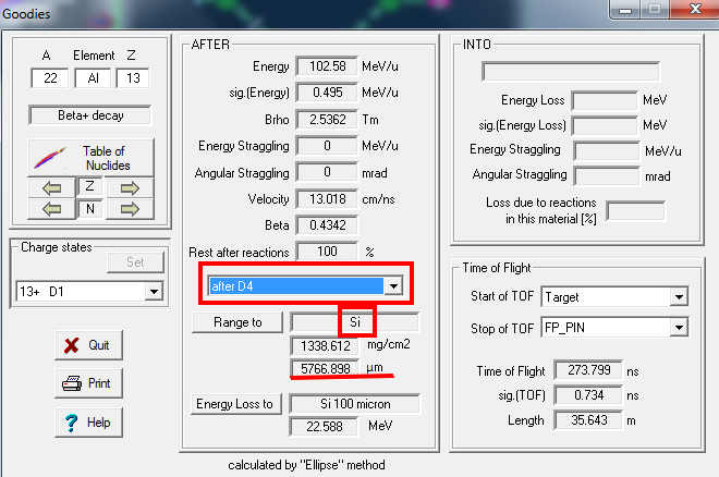
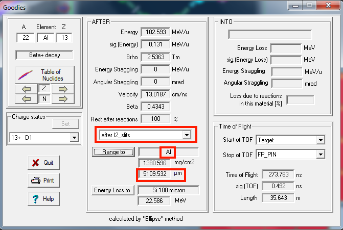
The goal is to change Image2 ( I2_slits) setting to adjust the $dp/p$ such that $^{22}$Al beam range of spreading in detector within 100 $\mu$m. So we will image that the FP_PIN detector, which is a silicon detector, is thick enough to stop all the $^{22}$Al ions, and the proper I2_slits setting can let the range of the $^{22}$Al ions within FWHM $\approx 100\mu\textrm{m}$ . So let's use "Goodies" to calculate the $^{22}$Al ion's range in a silicon detector after magnetic dipole D4.
menu bar --> "calculations" --> "Goodies".


select the "D4" options
We get the thickness around 5767 $\mu$m.


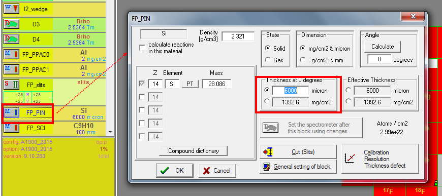
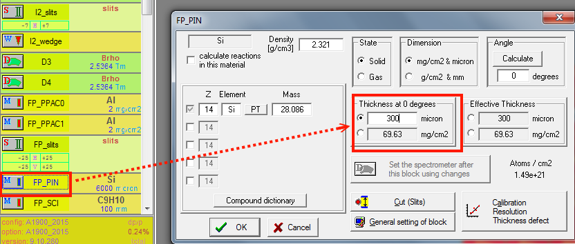
Next, we set the thickness of PIN detector at the Focal Plane to 6000 $\mu$m, allowing to fully stop $^{22}$Al.


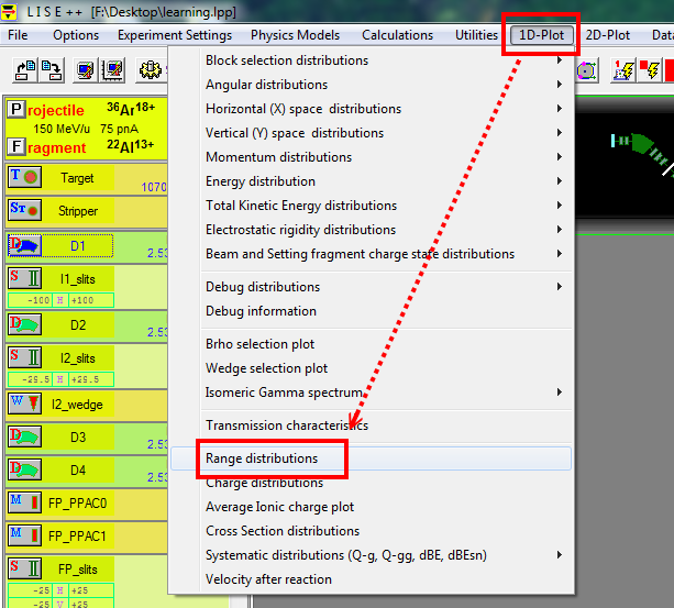
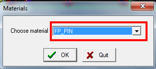
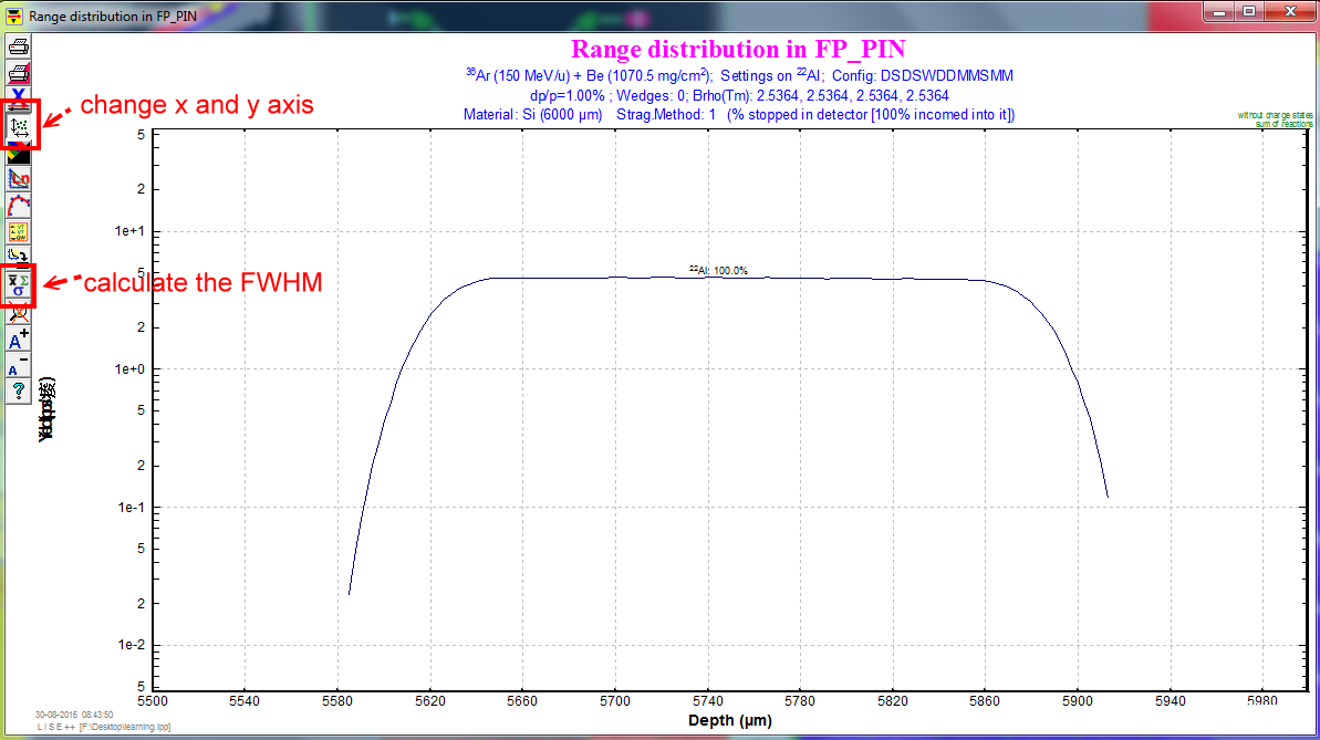
Let's check the range distribution plot of $^{22}$Al in the PIN detector.
menu bar --> "1D Plot" --> "Range distribution".



By click the button on the left-hand side, we find the FWHM is around 267.2 $\mu$m.
This is the current value, and we will change the "I2_slits" to make it $\approx 100\mu\textrm{m}$.

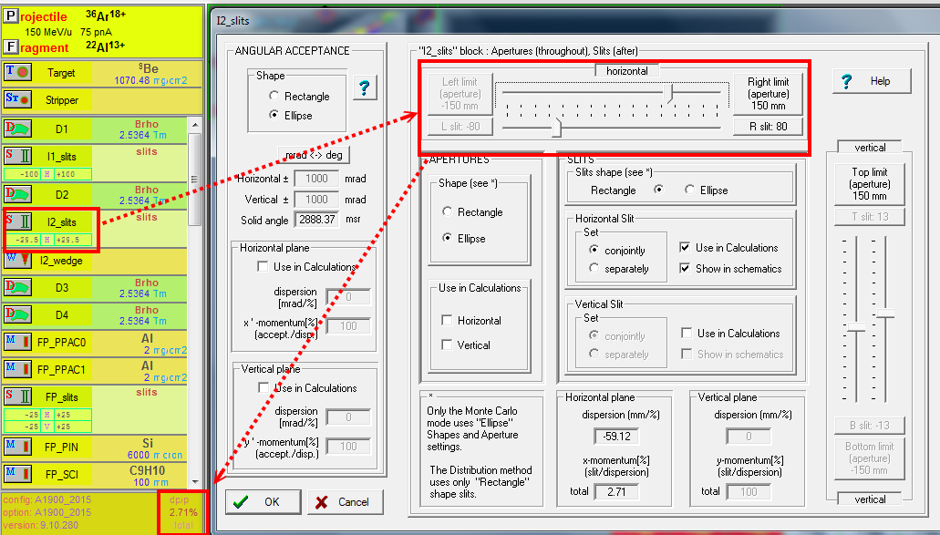
Adjust the Image2 (I2_slits)

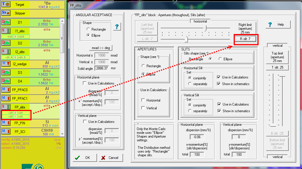
I2 slits are horizontal slits at the dispersive focal plane, it is to change the momentum acceptance $\frac{dp}{p}$. Its default horizontal slits are set to $\pm$ 150$mm$ (fully open), and let we change it to 7. And we can see the $\frac{dp}{p}=0.24\%$ now. Redo menu bar --> "1D Plot" --> "Range distribution", we can see the FWHM $\approx$ 100 $\mu$m in the 1D range plot.



Now we done with our momentum acceptance setting, we should reset the thickness of "FP_PIN" detector, so that it would not stop the $^{22}$Al beam anymore. Let's use 300$\mu$m.

Part 4 : $\Delta$E-TOF identification plot

Before having the plot, we need to calculate the transmission and rates, and then we can have data to plot.
menu bar --> calculations --> transmission and rate --> all nuclei.
Of course, we can manually "double right click" the elements in the chart to do the calculations.
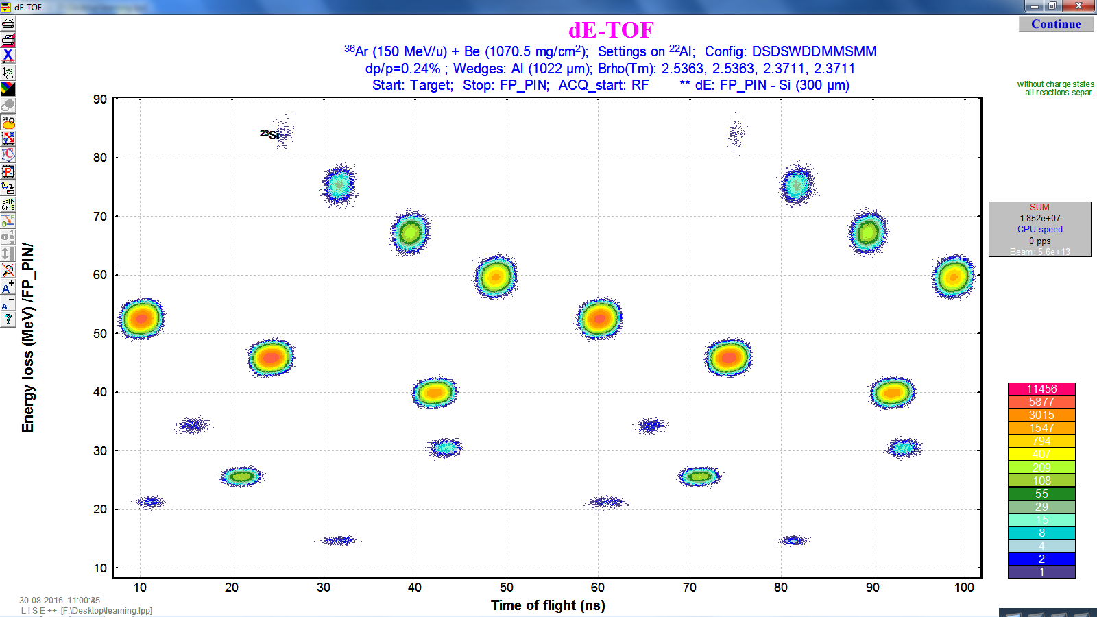
then menu bar --> 2D Plot --> Plot dE-TOF.



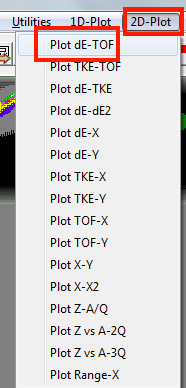
The result will look like the following figure.
Y axis is the energy loss in FP_PIN detector (300$\mu$m Si detector),
X axis is the TOF is the time of flight from target to FP_PIN in ns.



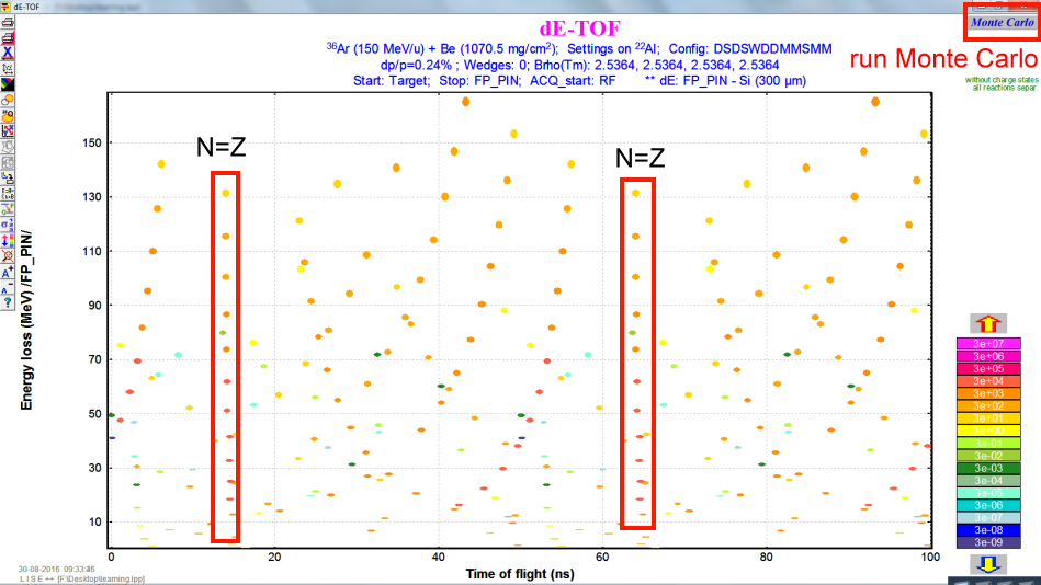
We can Run the Monte Carlo simulations, by press the upper right button.
One of useful thing is to do the channel calibration.

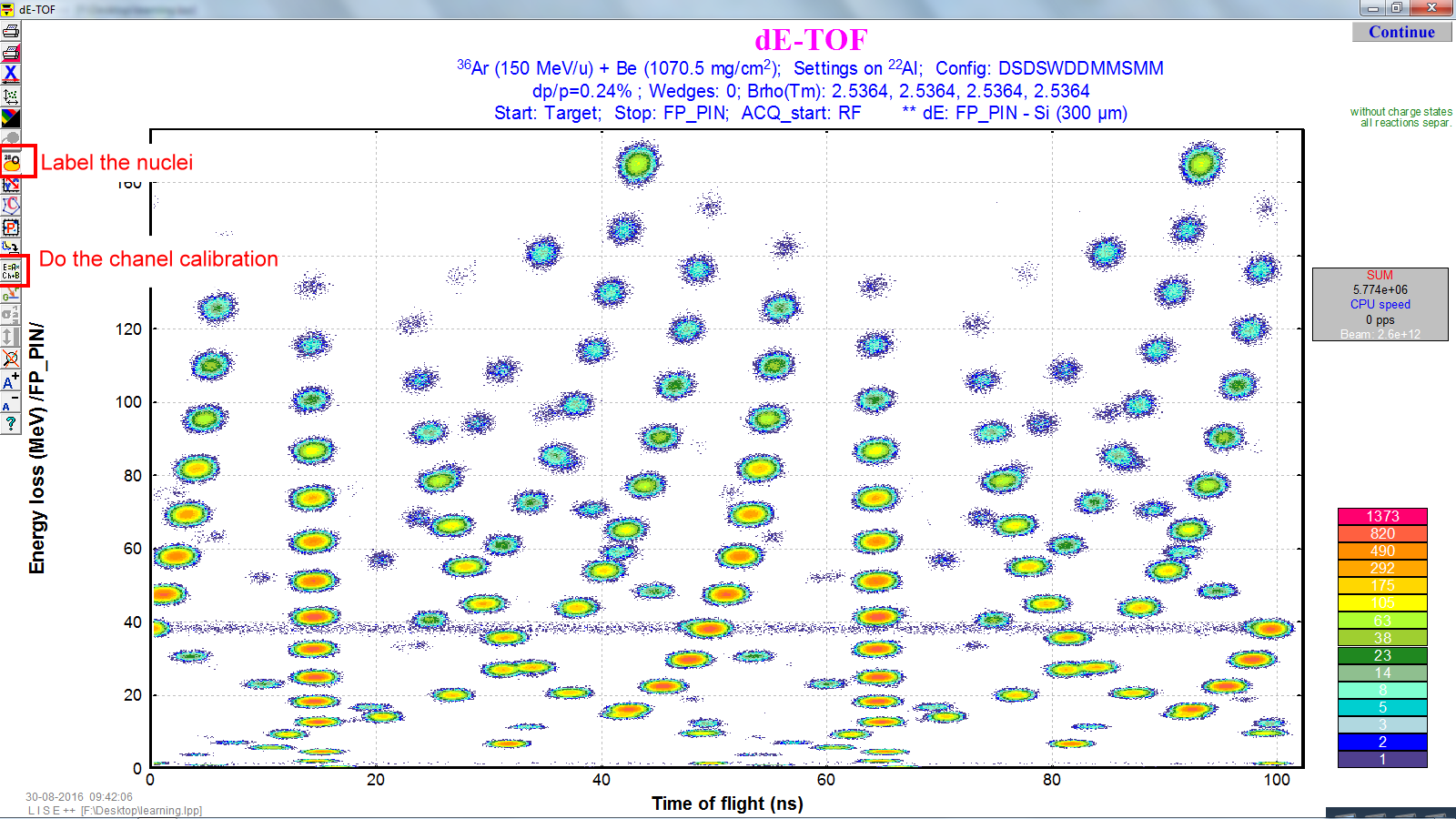
The rest of our jobs is to get rid of these unwanted contaminations in the secondary beams.

Part 5: Al Wedge setting

To eliminate or reduce the contaminations in the the secondary beams, one good idea is to use an achromatic wedge at the dispersive plane of the fragment separator. Because each nucleus will loose a different amount of energy in that wedge (Aluminum). Before setting the thickness for the Al wedge, we need to have some reference to know how good or bad our setting is, so we will use $B_\rho$ selection plot.
menu bar --> 1D Plot --> Brho selection plot.



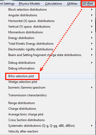
The results are like the following graph, x axis is $B_{rho}$ and y axis is yield (in log scale).
The red line is for $^{22}$Al.



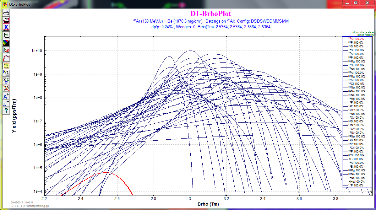
According to Dr. Bazin, a good rule of thumb is to set the wedge thickness to roughly 20% of the total range of the desired fragment. So I think that is the 20% of the total range for a $^{22}$Al in the Aluminum. Again, we can use Goodies to calculate its range. And I select after I2_slits. (This part I am not 100% sure). The calculations show the range around 5110$\mu$m, and 20% will be 1022$\mu$m.



So let's set the thickness of wedge. And then we need to press the button of "Set the spectrometer after this block using changes". Then check the box of wedge profile, then press the button of calculate angle.



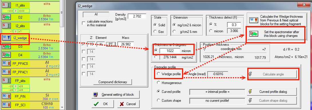
In the popping out window, press the "Fix". (The GUI seems different)



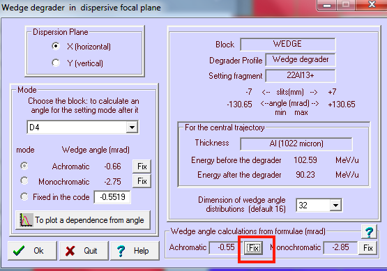
We can see a new wedge icon appears, and then we press the button to re-calculate the spectrometer setting.



Re-plot the $\Delta$E-TOF plot, we will see the difference.

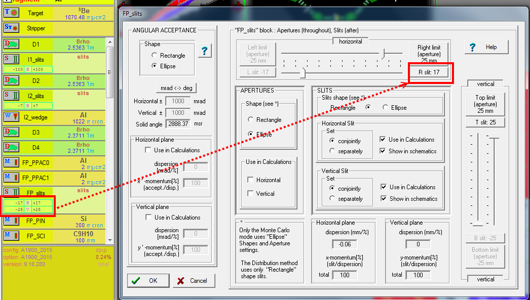
Part 6 : FP_slits seting

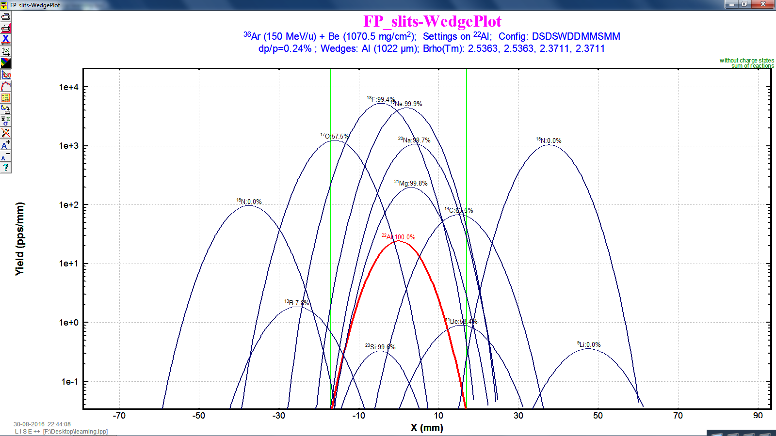
As being mentioned in part 4 to tune the "I2_slits" for momentum acceptance, we can also tune the "FP_slits" to do wedge selection for only allow our interested fragments to come through. So let's see the wedge selection plot first. Make sure you have done "transmission and rate" calculation.
menu bar -> 1D-plot -> Wedge selection plot.



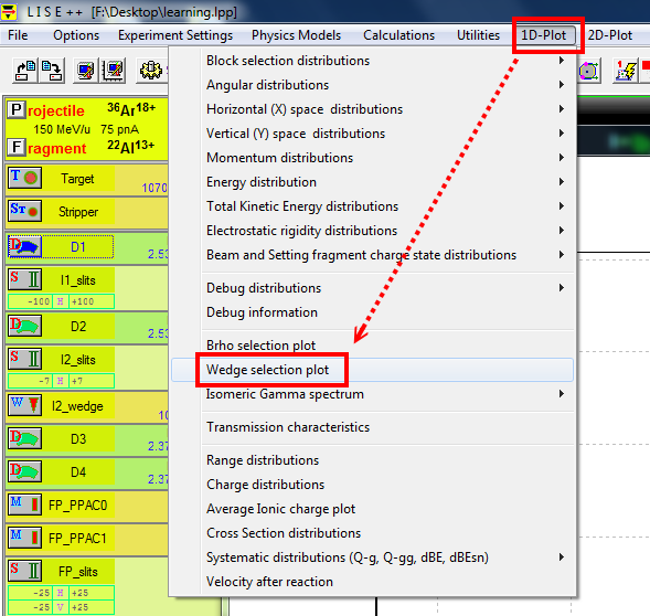
The result is the following graph. The x axis is the fragment position and y axis is the yield.
We want to move the green bar (the slits setting) as close as to the red curve.



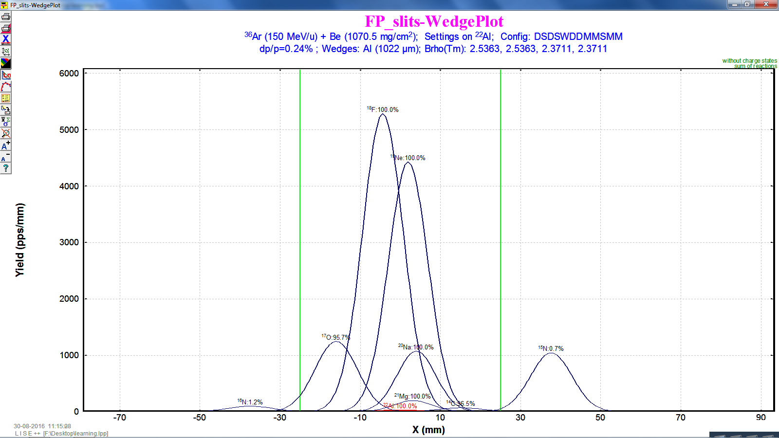
Now I set the horizontal opening of the slits to 17mm .


Then we re-run the "transmission and rate", and then re-plot "wedge selection plot" to check our setting.
Note: the graph is in the log scale.

Part 7 : adding new blocks

The next thing to improve our beam is to add a Wien filter and a compensating dipole (for re-focusing) before the "FP_PIN" detector, in order to separate the isotones.
menu bar icon-> set-up -> check "FP-PIN"
And then insert the "Wien velocity filter" and " compensating dipole".



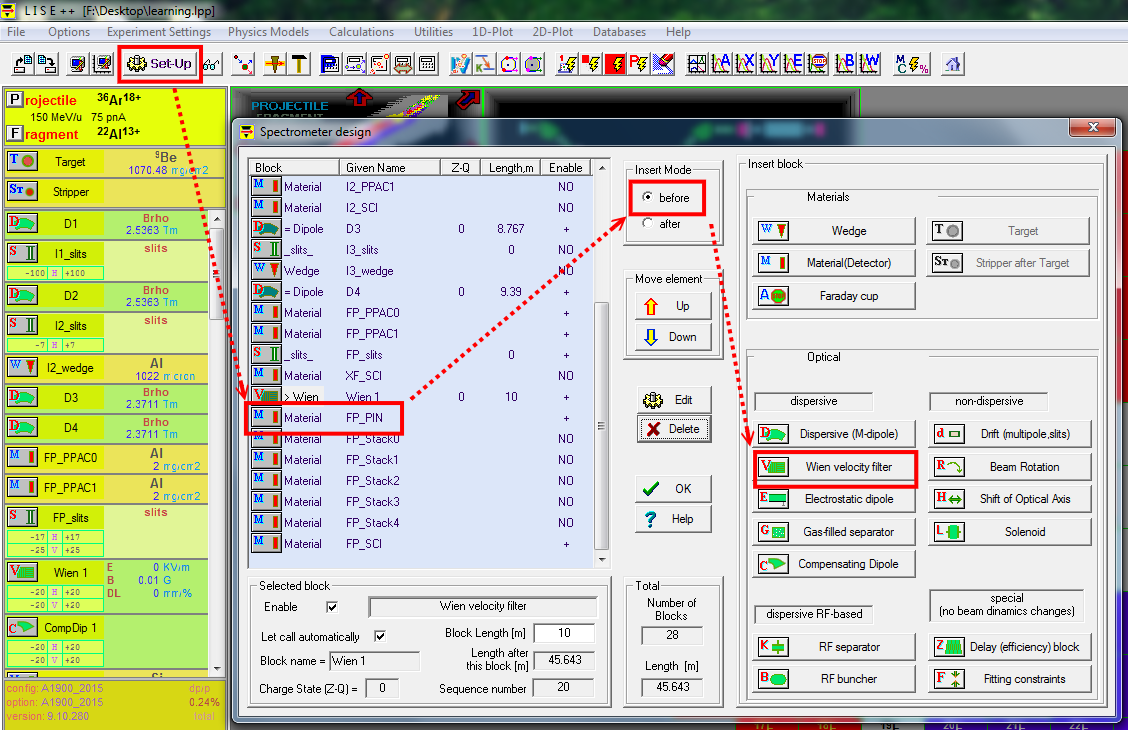
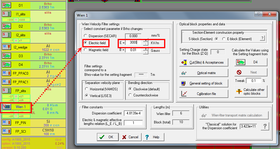
After adding the new block, we set the Electric filed to the "Wien velocity filter"
The E field is in the y direction. Now the fragments will have some y-direction deflection after the Wien filter, and hence we can close our slits of compensating dipole to allow $^{22}$Al to pass.



Let's see the fragments into the compensating dipole.
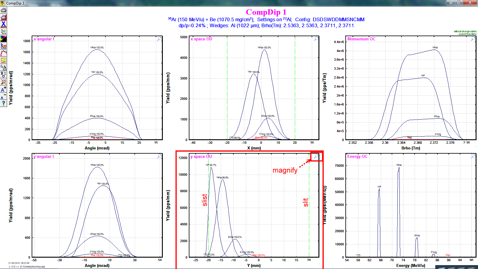
By 1-D plot, then select "Block selection distributions", and then "compDip1".



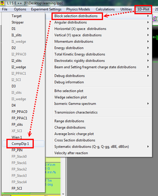
The results are following. Check the Y-space graph in the middle since our E field is in the y direction. Next thing is to close the slits to proper length. Its process is very similar to closing the I2_slits or FP_slits, and hence I skip this demonstration.

Quick guide

This demonstrate here follows from the guide written by Tom Ginter. The main point here is to set specific beam energy. The main difference is the order of "9Be target thickness optimization" and "Al wedge thickness". Here we set the thickness of the Al wedge first, then optimize the thickness of 9Be target.


For convenience, we keep discussing the same $^{22}$Al.
(1) set $^{36}$Ar for the projectile and $^{22}$Al for fragment.
(2) click I2_slits and set 800 mg/cm^2 for Al wedge.
Note: according the guide, for $1 \lt Z_{fagment} \lt 15$, use 800 mg/cm^2 for Al wedge.



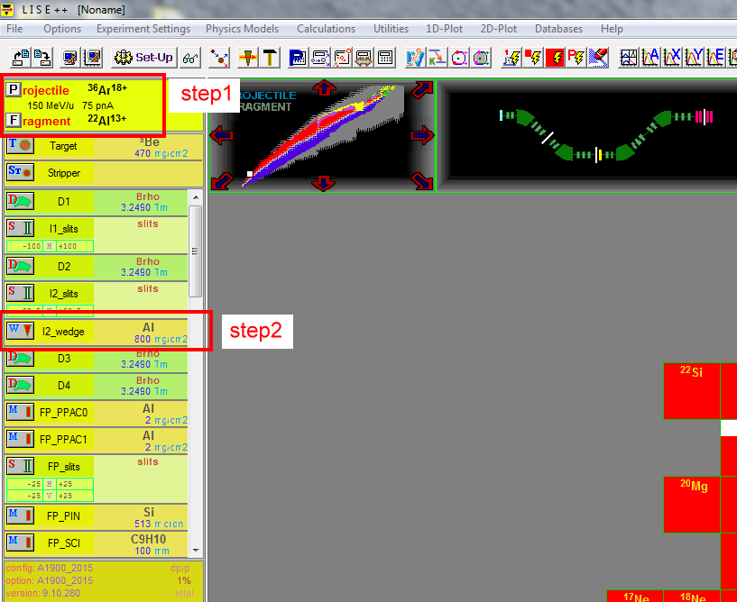
Suppose we want 40 MeV/u for our beam, which is the energy after magnetic dipole D4.
(1) We call "physical calculator" to convert MeV/u to magnetic rigidity (momentum/charge) in the unit of Tm. And then (2) Copy this number to D4.

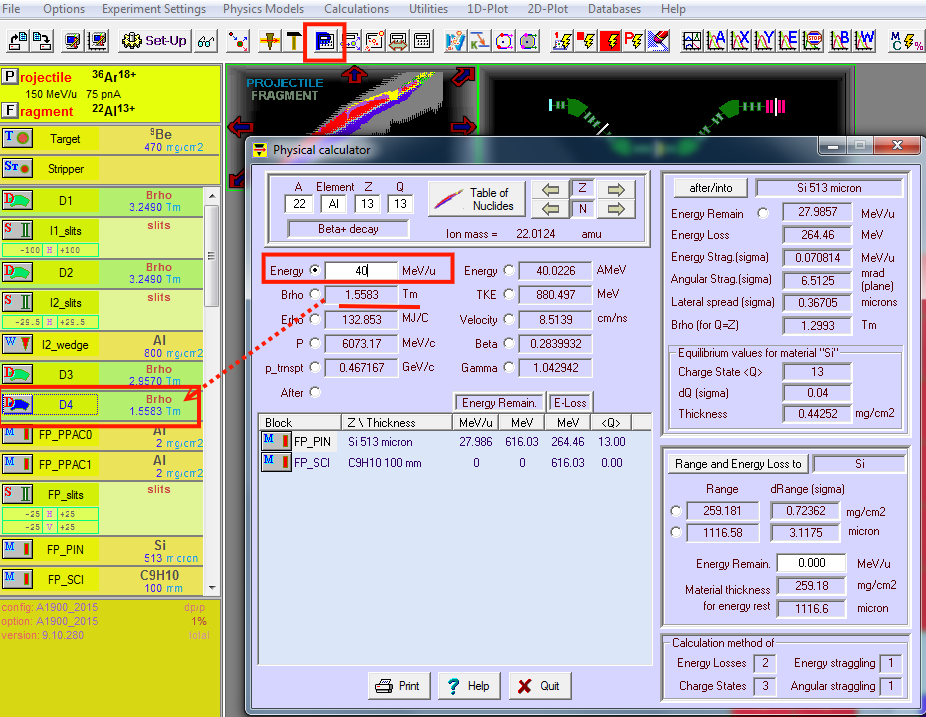
ps. the D4 is good approximation, maybe in your beam line, you have some other stuffs (ex. object scintillator ) which can reduce your beam energy. The NSCL beam physicists will tell you more. Your LISE++ calculation can provide a preliminary simulation.

Now, (1) run the target thickness optimization, and
(2) keep to D4. Copy the optimal thickness to the target. Then,
(3) run rigidity calculation (to tune rigidity).



YOu can further play around the horizontal FP_slits. $\pm$25 mm is is appropriate for experiments taking place at the A1900 focal plane, and $\pm$25 mm is appropriate for simulating rates. You can make the slit opening smaller, then you have smaller momentum spread (dp/p).



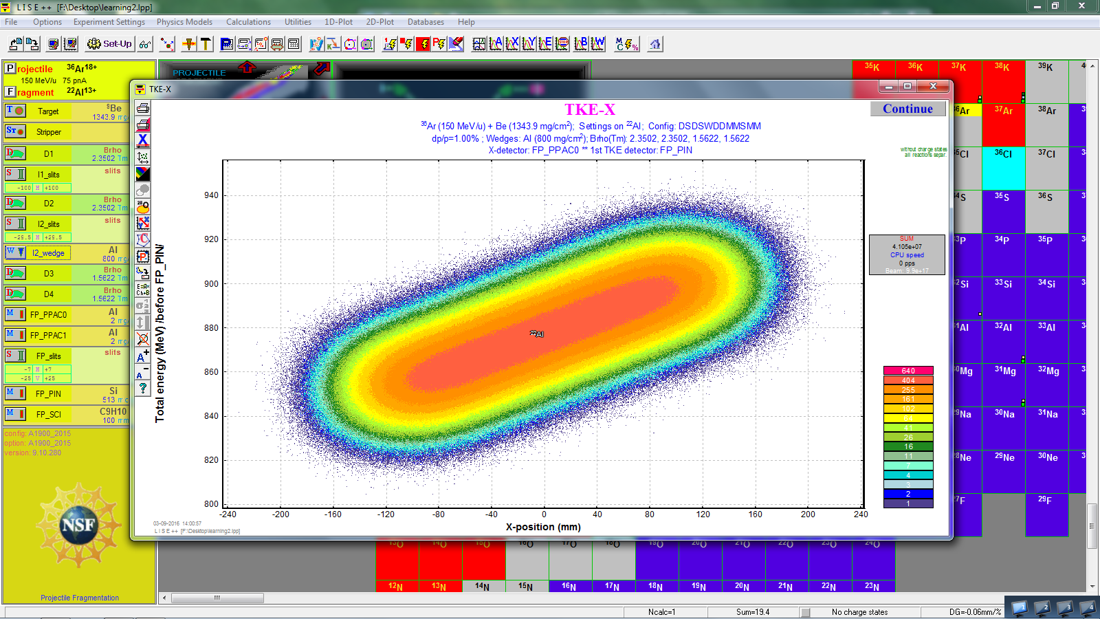
Just for checking. We should not have an appreciable correlation between position and total kinetic energy. To check it (1) 2D-plot -> Plot TKE-X (2) run Monte Carlo.
If the correlation appears, we need to adjust the wedge (its angle).



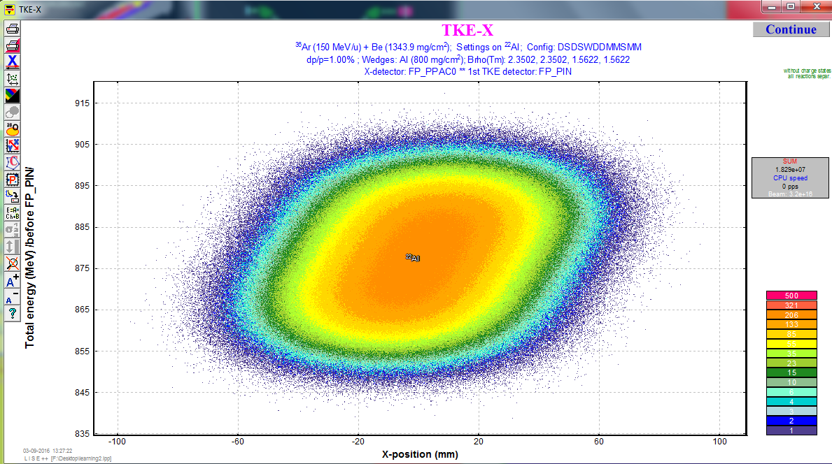
For example, let try to mess up the setting, for example set the angle to -5.



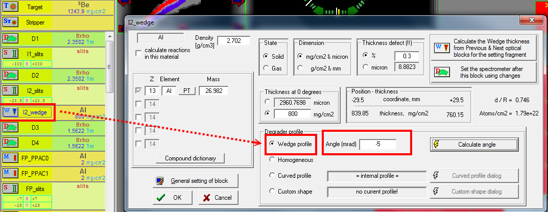
Then we see the correlations between position and total kinematic energy.


note:
The parameters we frequently change are:
(I) Al wedge thickness (angles),
(II) I2_slits and FP_Slits setting,
(III) Be target thickness.
Thinner wedges lead to smaller spot sizes for individual isotopes;
thicker wedges lead to a wider position separation between different isotopes.

Larger I2 slit settings give higher rates (up to limit of 5%) but scarifies the isotopic resolution on the basis of $\Delta\textrm{E-vs-TOF}$ measurements; settings of 1% or less are usually necessary to maintain particle identification resolution without resorting to particle-by-particle momentum correction techniques.

Barney printout

The NSCL Barney printouts are the beam setting data, and they are available at here.

The following is an example from the beam line to the S3 valut with the S800 spectrograph. We can see the rigidity setting for each beam line segment. These are real setting, not the simulated ones. The last one, Set 8, is the rigidity setting inside the S800 spectrograph. It is usually optimized for the recoils after the reaction of experimentalist's interest. The rigidity in Seg 7 should be the beam energy before the target.


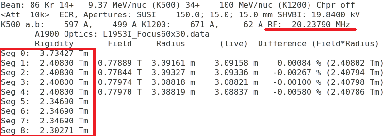
The rigidity changes between seg 4 and 5, since there is a plastic scintillator there (called XFP) so that the beam energy changes. Meanwhile, there could be another plastic scintillator between Set 5 and 6 (call object scint.). We can put the rigidity at Seg 4 into the D4 value in the LISE++.