• Profile
• Physics
• Programming
• Tutorial
• More
  • link 1
  • link 2
  • link 3

Part 1:Download And Installation

The current version is 4.11, and the source code can be download here (vikar4.tar).

tar xf vikar4X.tar to untar the file.
And there will be "sermon.txt" and "note.txt" to help users.
Inside the "source" folder, type in make, then it will generate executable "vikar".

If there are error messages during the compilation, such as:
make: f77: Command not found
make: *** [cart2sphere.o] Error 127
you can uncomment the line in Makefile:
#FC = /usr/bin/gfortran
If this does not work, then you need to check the path for your gfortran compiler.

ps. The new part for 4.11 version is it includes the simulation if we using beam tracking device. It will generate output files with '_recon' suffix. Beam tracking devices, like two MCPs, can increase the incoming beam position resolution, such that we can have a better angle information between the ejectile and the beam axis.

Part 2: Input

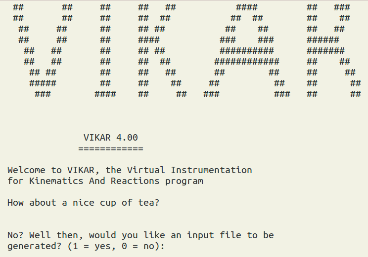
Run the code by ./vikor, VIKAR will guide you to input a series of parameters.

First, VIKAR as us whether we would like to write out a summary of our inputs. Yes, we do need it, and then give a name for your input file.


Currently, we only support two-body reaction, and that is good enough for the $^{2}$H($^{126}$Xe, $p$)$^{127}$Xe reaction.



____Reaction data block____
//Enter the (Z,A) information for beam, target, and ejectile:
Beam = $^{126}$Xe, with Z = 54, A = 126.
Target = d, with Z = 1, A = 2.
Ejectile = p, with Z = 1, A = 1.


/*
note:, we type in "54" then enter, then "126" then enter.
for the Z and A for the beam.
Suppose you have whole target composition is CD$_{2}$,
but the reaction is for $^{126}$Xe + $d$ only,
and therefore you should only use the Z=1 and A=2 for $d$.
*/

//Then you will enter beam information:
Beam energy = 1260.0 MeV. (10 MeV/A )
Beam spot size FWHM = 2.0 mm .
Beam energy spread FWHM = 2.52 MeV .
Beam divergence FWHM = 0.5 deg.


/*
note: for stable beam, normally, the beam size is around 2 mm.
For radiative beam, the beam size is larger. It can be a rectangular shape, height = 15 mm, width = 10mm.
The beam energy spread depends on the beam setting. (ΔE/E ≃ 2 * Δp/p).
If your momentum acceptance is 0.1%, then you have energy in 0.2%.
beam divergence is the incidence angle divergence. If it is 0, the beam is totally along the beam axis.
In reality, it can be somewhat off the beam axis.
*/

position resolution after beam tracking reconstruction = any
angle resolution after beam tracking reconstruction = any
//If we don't use beam tracking device, then just input any number.


____Block 2____
Then you will enter reaction information:
Ground state Q-value = 5.02 MeV
// Note: Q-value can be calculated from LISE,CATKIN, or NNDC online calculator.
// For LISE: Menu bar -> calculations -> calculator -> Kinematics Calculator.

Number of states populated in the residual = 3 (up to 20):
Excitation energy of state 1 in residual = 0.0 MeV.
Excitation energy of state 2 in residual = 1.0 MeV.
Excitation energy of state 3 in residual = 2.5 MeV.
// These are just hypothetical states.

____Block 3____
Then we give angular distributions ($\frac{\textrm{d}\theta} {\textrm{d}\Omega}$) of the ejectile:
// we can use the relative file path
// angular distribution is calculated from TWOFNR or Fresco.
// it takes the CM angular distribution.
// it takes two-colunm type data, ( CM angle, $\frac{\textrm{d}\theta} {\textrm{d}\Omega}$)
filename for ang. dist. profile for state 1 in residual = gs.xxx
filename for ang. dist. profile for state 2 in residual = Ex_1.xxx
filename for ang. dist. profile for state 3 in residual = Ex_2.xxx


____Block 4____
Then the detail composition of the target:
// for inverse (d,p), we generally use Cd$_{2}$ target, it has one $^{12}$C and two $^{2}$H.
Number of different elements in target molecule = 2 .
// for $^{12}$C
Z of element 1 = 6.
A of element 1 = 12.
atoms of element 1 per molecule N of atoms of element per target molecule = 1.
// for $^{2}$H
Z of element 2 = 1.
A of element 2 = 2.
N of atoms of element per target molecule = 2.


// Cd$_{2}$ target
Target thickness (mg/cm$^{2}$) = 0.2
Target density (g/cm$^{3}$) = 1.06300
Target style = 1 //foil = 1, jet=2
Target upstream backing = 0    // yes = 1, no = 0
Target downstream backing = 0   // yes = 1, no = 0
Foil target angle (degrees) = 0.0


____Block 5____
Range calculation which related to stopping power d$E$/d$x$.
// internal function = 0, external data = 1
// here we can type in 0 all the way.

beam particle range tables = 0

// in Target
ejectile range tables in TARGET = 0
recoil range tables in TARGET = 0

// in Detector
ejectile range tables in DETECTOR = 0
recoil range tables in DETECTOR = 0


____Block 6____
The detector data set is under the detectors directory.


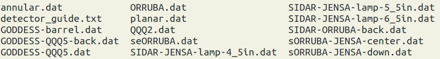
perfect (0) or real (1) detectors = 1
filename for cylindrical detector setup file = GODDESS-barrel.dat
filename for planar detector setup file = none
filename for annular detector setup file = GODDESS-QQQ5-back.dat


____Block 7____
perfect (0) or realistic (1) charge collection = 1
Number of events required to exit = 10000

//Output options: Yes = 1, No = 0
Detect ejectiles? = 1
Detect recoils? = 0

Write undetected ejectiles? = 1
Write undetected recoils? = 1
No formatting (0) or grace (1) for output files = 1

No (0) or automatic (1) Q-value calcualtions = 1
Q-value spectrum dispersion (channels per MeV) = 20.0

Part 3: Output

We will get a series of dat files, and we can use xmgrace to open them.

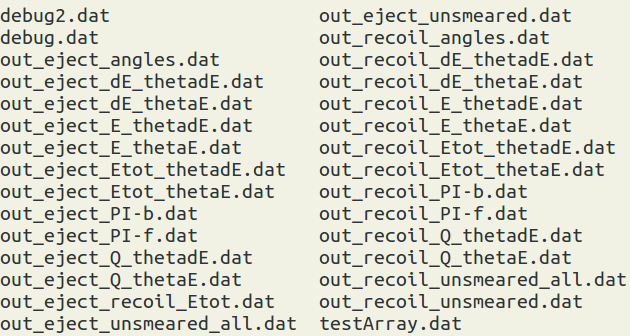
Naming rule: out_[particle type]_[energy_type]_[angle type].dat.
The particle type can be ejectile or recoil
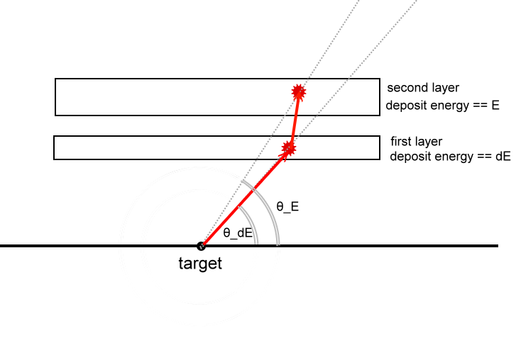
The energy types have three options: E , dE , Etot (=E +dE)
The angle types have two options: be $\theta_{dE}$ or $\theta_{E}$

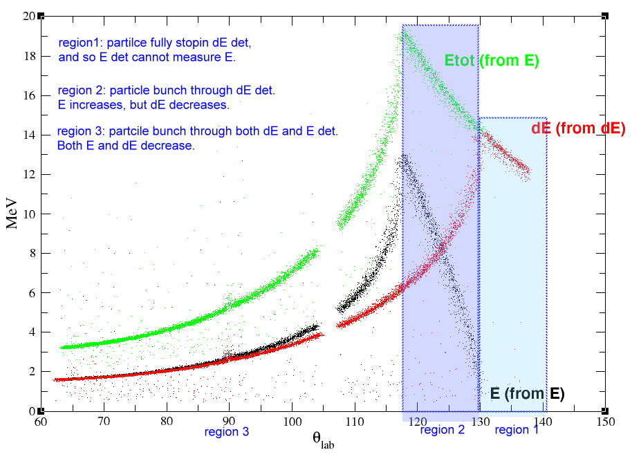
Conventionally, a telescope have two layer, first layer we call dE detector, and the second layer is the E detector. We specify the energy measured from the first layer (usually thiner) as "dE", and the energy measured in the second layer as "E".

The angle has two different definitions, since the particle can interact with the first layer and then changes its path. Also if the particle is fully stopped in the first layer, we can have only $\theta_{dE}$, but there will no $\theta_{E}$ information. Also if we artificial set the first layer to 0.001 $\mu$m in thickness, which is too thin and the energy deposit will be approximately zero; it tells the program we don't have a dE detector.


The following are samples: "out_eject_dE_thetadE.dat" is the graph with the x axis as $\theta_{lab}$ and the y axis as the energy deposit to the dE Si detector for the ejectile. "out_eject_E_thetaE.dat" is the graph with the x axis as $\theta_{lab}$ and the y axis as the energy deposit to the E Si detector for the ejectile. "out_eject_Etot_thetaE.dat" has x axis as $\theta_{lab}$ and the y axis as Etot from the E detector for the ejectile.

Note: Files containing "_unsmeared" include beam and target effects only (ie no detector resolution effects). Files as "*_angles.dat" contain a hit map of the particles in "spherical polar coordinates."

part 4 : detector guide

Note that, for cylindrical geometry, resisitve and non-resistive detectors can be simulated. For resistive detectors, energy-dependent (with 1/E) position resolution and energy-dependent thresholds are simulated.



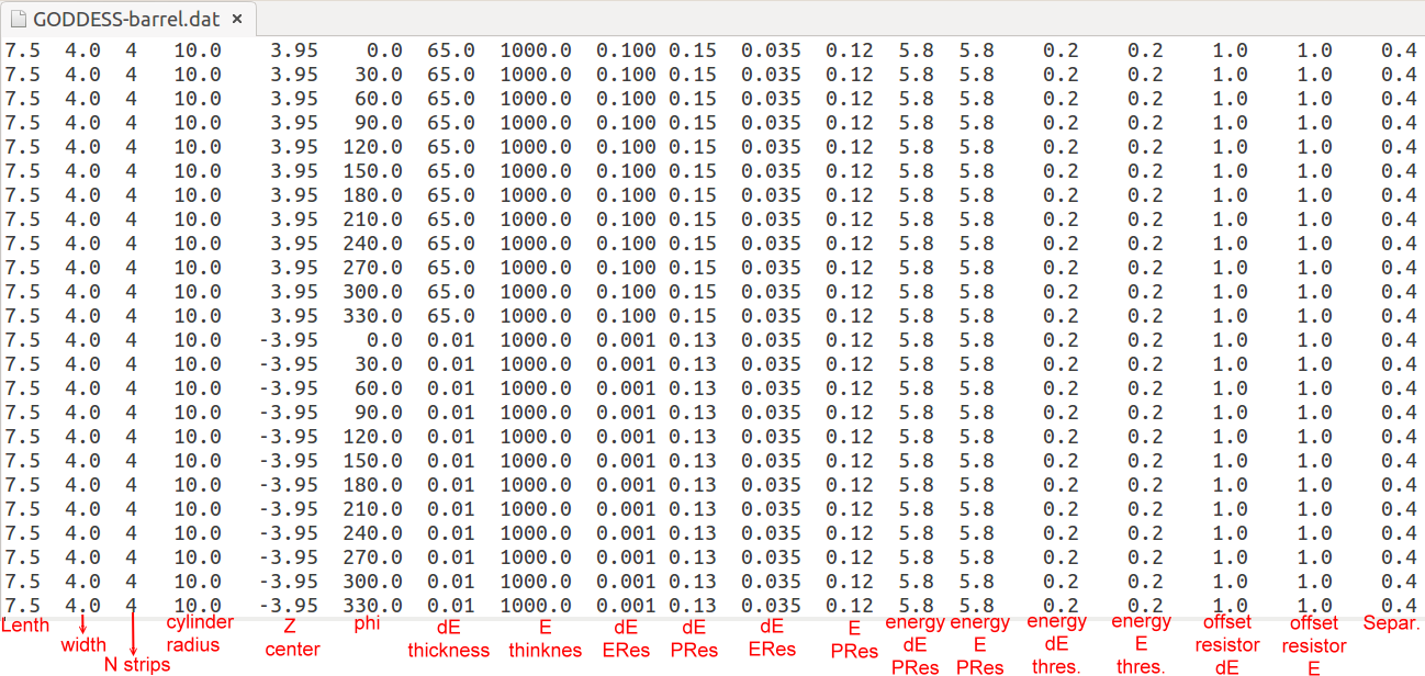
Cylindrical Geometry (19 parameters)
--------------------

Telescope Length (cm)
Telescope Width (cm)
Number of Strips
Cylinder radius (cm)
Telescope Center along Z (cm)
Telescope Phi (deg)
dE Thickness (um)
E Thickness (um)
dE Eres (MeV)
dE Pres (at 5.8 MeV) (cm)
E Eres (MeV)
E Pres (at 5.8 MeV) (cm)
Energy of dE Pres (MeV)
Energy of E Pres (MeV)
dE Energy threshold (MeV)
E Energy threshold (MeV)
dE offset resistors (k Ohm)
E offset resistors (k Ohm)
Telescope separation (cm)



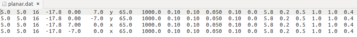
Planar Geometry (20 parameters)
---------------

Telescope Length (cm)
Telescope Width (cm)
Number of Strips
Telescope Z (cm)
Telescope centre X (cm)
Telescope centre Y (cm)
Strip orientation (x or y)
dE Thickness (um)
E Thickness (um)
dE Eres (MeV)
dE Pres (at 5.8 MeV) (cm)
E Eres (MeV)
E Pres (at 5.8 MeV) (cm)
Energy of dE Pres (cm)
Energy of E Pres (cm)
dE Energy threshold (MeV)
E Energy threshold (MeV)
dE offset resistors (k Ohm)
E offset resistors (k Ohm)
Telescope separation (cm)



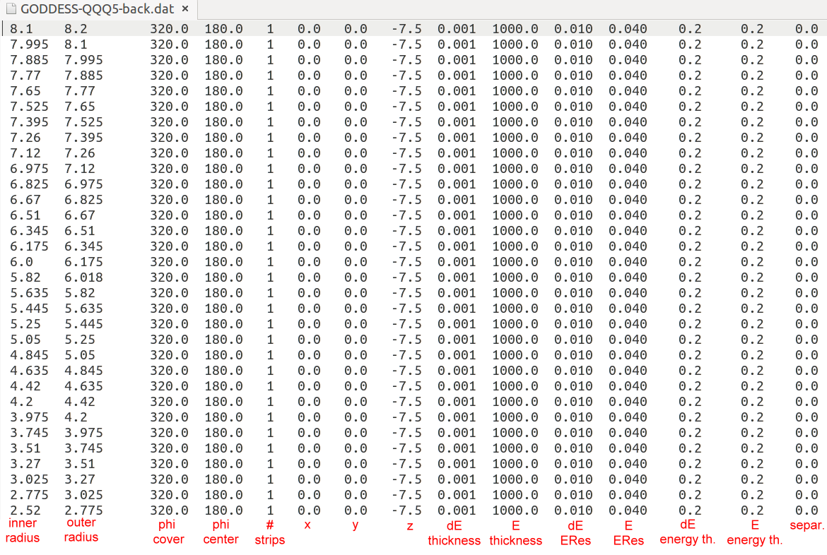
Annular Geometry (15 parameters)
----------------

Telescope Inner Radius (cm)
Telescope Outer Radius (cm)
Telescope Phi Coverage (deg)
Telescope Phi Centre (deg)
Number of Strips
Telescope X location (cm)
Telescope Y location (cm)
Telescope Z location (cm)
dE Thickness (um)
E Thickness (um)
dE Eres (MeV)
E Eres (MeV)
dE Energy threshold (MeV)
E Energy threshold (MeV)
Telescope separation (cm)

note: dE Pres (at 5.8 MeV) ==> the dE position resolution at the 5.8 MeV.
The alpha source ²⁴⁹Cf has a 5810-keV peak. So we simply call it 5.8-MeV peak.
The Cylinder and Planar detectors are set to be resistive, and so they have the ability to measure the position of a particle when it hits a resistive strip. A resistive strip will divide its charge to the two end, and so position is related to $\frac{V_{L}-V_{R} } { V_{L}+V_{R} }$ ( of course, one has to take care of gain matching and the offset for the signals from the two ends of a strip).

Energy of dE Pres ==> it is the energy we quote for the position resolution. It is 5.8 MeV for the alpha source we use. The position resolution of a resistive strip is energy dependent. The position resolution is worse for lower energy. When the position resolution of your detector doesn't have energy dependence, just set this term to 0.

Telescope separation is the distance between dE and E detectors.

offset resistors (k Ohm) ==> can be found from the manufacture's manual. This term determines how low a $V_{L}$ or $V_{R}$ can be measured. I.E. $V_{L}=0.0000000001 $mV may not be physically possible.