
Run the DSAM_GUI code
The program is installed in the polar server, under tabor2 account. You can login by tabor2 to copy the whole folder 'DSAM_GUI' to your home directory, and you are ready to run the code. Inside the DSAM_GUI, key in ./goDSAM, then you will see the GUI. ( If you need the source code to try your own, you are very welcome to email to me.)
Installation
If you want to install the program, you have to make sure that you have Python 2.7 or later, in which the PIL (python image library 1.1.7 for PNG files) library is supported. The Ubuntu 14.04 version will be all fine. Also the xmgrace program is needed to generate the png figures. If you don't have the xmgrace program. Type in sudo apt-get install grace to install it. And there are C++ and Fortran 77 programs to compile in the 'lib'. Go to the 'lib' folder, and then key in make to compile theses files.
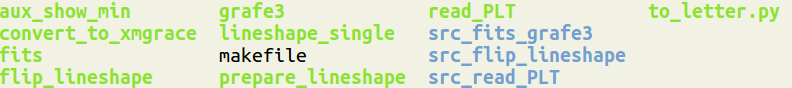
Figure: the files inside the 'lib' folder.
STP (stopping power) file Panel
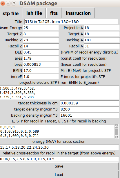
'stp panel' is located at the first tab from the left. Preparing a *.stp file is the first step to DSAM fitting. Generally speaking, creating a stopping power file (.stp) for DSAM fitting is NOT simple. You will need to run 'SRIM' for simulating nuclear and electric stopping power dE/dx (in the unit of MeV/ (mg/cm^2) ), and 'PACE' for simulating the 'relative' reaction cross-section. Additionally, you need to prepare certain information for the target; densities and thickness. This panel guides you to input the information. I already simplified the input and minimized the complexity.
The previous graduate student E.F. Moore wrote the 'Fits' program in Fortran 77 that need a stp file input. The details can be seen at his dissertation and Robert Kaye's dissertation. The following table explains the parameters. (sample)
| symbols | Original | DSAM_GUI | note |
| TITLE | 31Si in Ta 25 MeV | 31Si in Ta 25 MeV | (up to 30 characters) |
| AP | 18 | 18 | atomic mass for projectile (180 ) |
| EBMAX | 25 | 25 | max beam energy in MeV |
| ZT | 8 | 8 | proton number for target (18O) |
| AT | 18 | 18 | atomic mass for target (18O) |
| ZB | 73 | 73 | proton number for backing (181Ta) |
| AB | 181 | 181 | atomic mass for target (181Ta) |
| ZR | 14 | 14 | proton number for recoil (31Si) |
| AR | 31 | 31 | atomic mass for recoil (31Si) |
| IBALAU | 1 or 2 | (defult=1) |
1 = using Blaugrund's approximation, 2= no nuclear scattering |
| DEL | from 0 to 1 | from 0 to 1 | FWHM of recoil energy distribution = ? of max energy |
| NTHETR | from 0 to 5 | (defult=1) | number of recoil theta angles, max = 5 |
| NPHIR | from 0 to 10 | (defult=1) | number of recoil phi angles, max = 10 |
| ANGR | 0 | (defult=0) | not clear to me, but it seems we don't use it. |
| PROBR | 1 | (defult=1) | not clear to me, but it seems we don't use it. |
| ARES | 1.79 | 1.79 | the FWHM will increase as E increases |
| BRES | 0.000853 | 0.000853 | FWHM = ares + bres * E + cres * E^2 |
| CRES | 0 | (defult=0) | normally CRES is very small |
| SNOP | 1 | (defult=0) | Projectile stopping power normalization |
| EMIN | 17 | 17 | Minimum beam energy for stopping power of projectile |
| DEP | 1 | 1 | delta E of projection ( energy increment for stp) |
| NPP | 9 | (auto) | stp power energy ( E=17, 17+1, ..., 17 +8) < EMax=25 |
| STTP[NPP] | 3.511, 3.484, 3.446... | 3.511, 3.484, 3.446... | at 17 MeV, projectile electronic dE/dx = 3.511 in target, at 18 MeV =3.484 |
| NUMEL | 100 | (default = 100) | number of target division sections |
| TARTH | 0.000159 | 0.000159 | target thickness in 'cm' |
| NTP | 20 | (auto) | number of target and backing stp entries (see ESTOP, STP ) |
| SNOT[1] | 1 | (default = 1) | target stopping power normalization |
| RHOT[1] | 8200 | 8200 | target density (mg/cm^3) mg = milligram = 10^-3 g |
| SNOT[1] | 1 | (default) | backing stopping power normalization |
| RHOT[1] | 16601 | 16601 | backing density (mg/cm^3) |
| FE[1] | 1 | (default=1) | normalization for electronic stopping power only for target |
| FN[1] | 1 | (default=1) | normalization for nuclear stopping power only for target |
| FE[2] | 1 | (default=1) | normalization for electronic stopping power only for backing |
| FN[2] | 1 | (default=1) | normalization for nuclear stopping power only for backing |
| NCHOICE | 1 or 2 | (default=2) | 1 = Kalbitzer and Oetzmann, 2 = Bohr's ansatz |
| 0, 0, 0, 0 | 0, 0, 0, 0 | ESTOP[1][i] >> STP[1][i] >> ESTOP[2][i] >> STP[2][i] | |
| 0.1, 0.951, 0.1, 0.61 | 0.1, 0.951, 0.1, 0.61 | at 0.1 MeV, elect. stp for recoil in target = 0.951 (MeV/ (mg/cm2) ), in backing = 0.61 | |
| 0.3, 1.094, 0.3, 0.77 | 0.3, 1.094, 0.3, 0.77 | at 0.3 MeV, stp for recoil at target = 1.094, at backing = 0.77 | |
| ... | ... | ||
| 35, 8.009, 35, 6.04 | 35, 8.009, 35, 6.04 | total NPP=20 entries | |
| NSIG | 8 | (auto) | number of cross-section entries |
| EBX[] | 15, 17.5, 18, ..., 30 | 15, 17.5, 18, ..., 30 | beam energy in MeV |
| SIGR[] | 0.06, 0.5, 2, ....10.5 | 0.06, 0.5, 2, ....10.5 | in 15 MeV, reaction 'relative' cross-section = 0.06 |
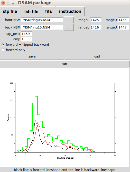
LSH (line shape) file Panel
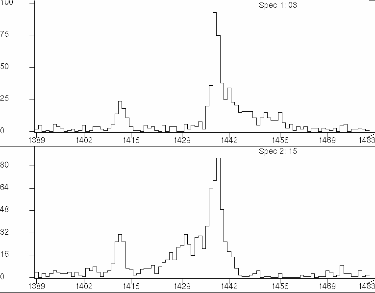
The next thing is to prepare the line shape of the peak you want to fit. Therefore, you need to sort the γ-γ matrix with an axis setting of all angles vs. a specific angle. For example: ring03.NSM is the histogram from the 30-vs-all γ-γ matrix. ring15.NSM is the histogram from the 150-vs-all γ-γ matrix. You can consider only to fit 30 deg line shape, or to fit a line shape with 30 deg + flip 150 deg, which is flipped in respective to the stopping peak position. In this example, the stopping peak position is at 1439 channel. You can also use the 90-vs-all γ-γ matrix to find the stopping peak position.
Once you generate the NSM files, the next thing is to gather the information for the 'fits' program. The original process is very tedious, such as you have to convert the channel number. It is inconvenient especially when you add forward and flip-backward line shapes. GSAM_GUI can make this process much easier.
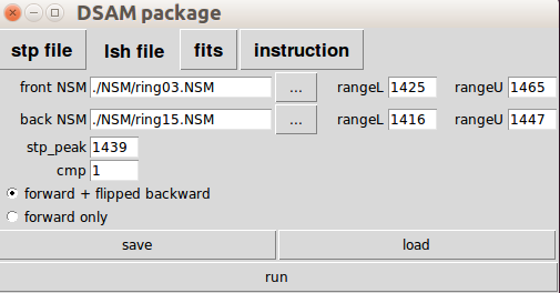
rangeL = lower limit of channel number
rangeU = upper limit of channel number
stp_peak = the stopping peak channel number
cmp = compression factor
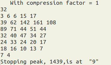
You have a set of two radio buttons to control the output. You can save and load the setting (default is to lineshape.lsh ). When you hit run, the output will show on the terminal as well as to lineshape.dat by default. Also the output will show on the terminal as well. And you can also edit the lineshape.dat file, such as when you want to certain data points. You can manually set them to '-1'.
fit (DSAM fitting) Panel
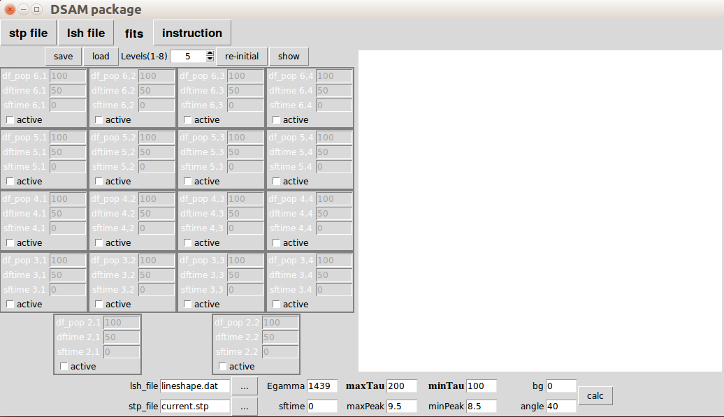
The 'fits' panel is the main part you will spend most of the time in DSAM. It provides visualization of feeding patterns and the fitting results. When you open 'DSAM_GUI' the default tab is 'fits' panel.
On the left is the units for feeding patterns.
On the right is for showing feeding patterns or showing fitting results.
On the bottom is the control for the fitting of the state of interest.
lifetime control section
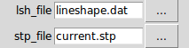
By default, the lsh file is set to lineshape.dat.
By default, the stp file is set to current.stp.
Once you change the lineshape.dat in the 'lsh file' panel,
You should reload the latest lineshape.dat file by the '...' button, and the program will parse the lineshape.dat and automatically set the Egamma, compression factor, minTau, and maxTau.
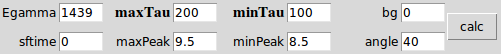
Egamma = γ-ray energy (in keV), we will use the stopping peak channel.
bg = background
angle = the angle for the forward line shape.
minTau = min tau for the state of interest (in fs).
maxTau = max tau for the state of interest (in fs).
I set the step is 10, and then d = (maxTau - minTau)/10. The 'fits' program will fit this state with tau from tau, tau + d, tau +2d, ..., tau + 9d
minPeak = the min stopping peak position in relative channel
maxPeak = the max stopping peak position in relative channel
I set the step is 5, and so when reading lineshape.dat, it will set:
minPeak = stp_peak - 0.5
maxPeak = stp_peak + 0.5
You can manually change them as well.
sftime = side feeding time (in fs) for the state of interest.
you can key in multiple values to fit and separate them by ','. For example: 0, 100, 200
The 'calc' button is for calling 'fits' program,
feeding pattern section

At the top is a control bar
the spin list is for the levels of feeding pattern (default = 5)
'save' = save the setting ( by default myDSAM.set )
'load' = load the setting ( by default myDSAM.set )
're-initial' = to reset and re-adjust the levels
'show' = to show the feeding.
If you already run the 'calc' button, you can use 'show' button to alternate the plots between feeding patterns and fitting results.
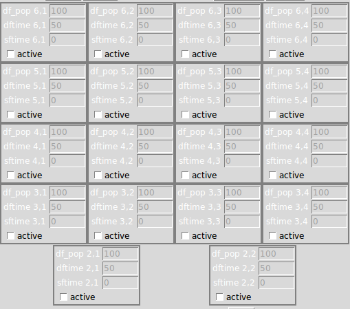
When setting the feeding pattern, check the box to activate the unit. There are four columns representing the four branches. The rows represent levels. The numbering system is a little bit wired, since I have to map it to the origin 'fits' program.
the state of interest is labeled as (1,2), at level = 1
then next are (2,1) and (2,2) at level 2
then next are (3,1) , (3,2), (3,3), (3,4), at level 3
See the following graph from E.F. Moore.
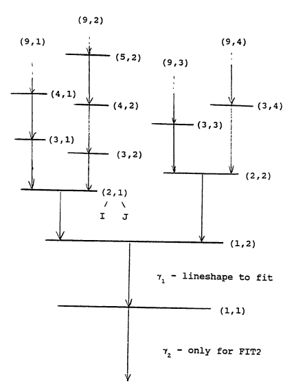
DSAM_GUI makes your work easier by showing the feeding patterns.
'df_pop' = direct feeding relative population (0-100)
'sftime' = side feeding time (in fs. )
'dftime' = side feeding time (in fs. )
you can input multiple value in the entries of'df_pop', 'sftime', and 'dftime', and use ',' to separate them, such as 1,2,3. The DSAM_GUI program will pick up the combination with minimum chi square value to plot. When you have multiple values, the canvas will only show '...'. If sftime = 0, it won't be shown in the canvas. See the following demonstration
Example 1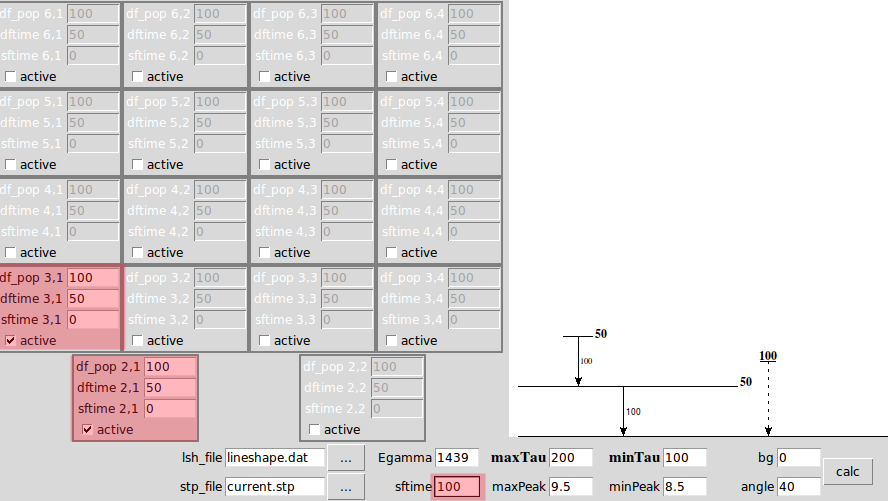
Example 2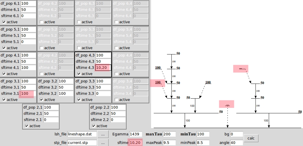
Example 3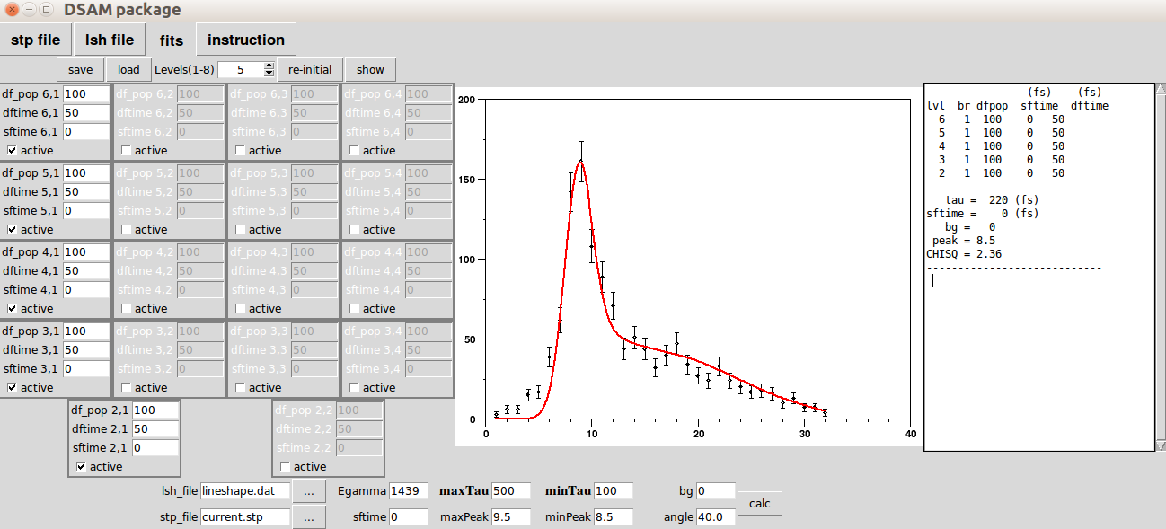
When you finish setting up the feeding patterns and lifetimes, hit the 'calc' button. It will show the following plot with the report on the most right windows, serving as your notepad. You can copy or edit the text there. In the following is a summary of line shape file, (sample )
Line Shape File
| simbols | note | |
| title | 1439a | 'DSAM GUI' will prepare it for you |
| ICH1 | 1 | 'DSAM GUI' will prepare it for you |
| ICH2 | 44 | 'DSAM GUI' will prepare it for you |
| ISPECE[] | 729 747 853 -1 -1 | 'DSAM GUI' will prepare it for you |
| -1 -1 1408 1651 2314 | You have to manually change to -1 | |
| 4068 6438 7066 5059 3199 | if you want to ignore some data point. | |
| 2358 2065 1957 1878 1820 | ||
| 1709 1648 1536 1418 1230 | ||
| 6,1,100,0.000,0.050 | I,J,${dfpopIJ},${sftimeIJ},${dftimeIJ} | |
| 5,1,100,0.000,0.050 | 'DSAM GUI' will prepare it for you | |
| 4,1,100,0.000,0.050 | 'DSAM GUI' will prepare it for you | |
| ... | 'DSAM GUI' will prepare it for you | |
| 1,2,100,0.000,0 | 'DSAM GUI' will prepare it for you | |
| 1,1,0,0,0 | 'DSAM GUI' will prepare it for you | |
| EGAM | 1439 | Gamma-ray energy = Stopping peak channel |
| THETA | 40 | Forward angle |
| A2 | (default = 0.01) | The A2 and A4 value is from angular distribution |
| A4 | (default = 0) | Normally they only have little influence. |
| TAULO | =minTau | |
| TAUHI | =maxTau | |
| DTAU | (auto) | set to only 10 steps |
| PKLO | =minPeak | |
| PKHI | =maxPeak | |
| DPEAK | (auto) | set to only 5 steps |
| IBKG | = bg | |
| ECAL | (auto) | = cmp (compression factor), retrieve from lineshape.dat |
| R | *(default = 3.5) | radius of Ge detector in cm (in this case GAMMASPHERE ) |
| H | * (default = 8.5 ) | thickness of Ge detector in cm |
| D | * (default = 25 ) | distance between target and detector in cm |
| NRAD | (default = 10) | Number of radial elements of the detector |
| NANG | (default = 10) | Number of angular elements of the detector |
| ( for correcting the finite solid angle.) |
Additional Information
The 'fits' program creates the summary document at fort.4 and fort.3. You can further utilize them to do your analysis. Furthermore the lineshape.dat file stores the line shape information. .A_script.sh is a hidden script to perform the 'fits' program. If you wish to have the source code, you are very welcome to contact me.
Contact: