
ROOTSCOPE Introduction
In a nutshell, ROOTSCOPE is a GUI application designed to deal with general CERN ROOT analysis for TH1 and TH2 histogram. ROOT package is very powerful, but somehow it is not efficient enough to my task. For example, doing gamma-ray analysis, one has to zoom in/out frequently and measure the peaks. The ROOT is not friendly in this task. ROOTSCOPE can use simple key and do the Gaussian fit, without writing any further script. ROOTSCOPE covers many functions I use for my research, and you are very welcome to suggest functions to add in the ROOTSCOPE. The current version is 2.0, and it has add more common used functions to deal with TH2. You can download the source code here or at my Github ( link ).
It is easier to understand how to use ROOTSCOPE by showing you the operation, and so please check out the following youtube clips. Aslo, in the menu bar, there are all the hot key combinations, and so you don't need to rememberer them.
There is also a lite version "ROOTSCOPE-lite". It is a workaround for older ROOT 5.xx version. Meanwhile, you can add shortcut keys to ROOTSCOPE or ROOTSCOPE-lite. It is easier to start from lite version, since it is shorter (and no confusing multipad stuffs).
The name of ROOTSCOPE is inspired by "Gnuscope", which is a software I used heavily during my Ph.D. study for gamma-ray spectroscopy analysis.
Quick start
You have to install ROOT version 6 or above to run ROOTSCOPE. (ROOT installation tutorial)
There are several methods to start the ROOTSCOPE application.
method 1:
to use the bash script "run_ROOTSCOPE.sh".You need to make this script executable.
(by
chmod 755 run_ROOTSCOPE.sh) ./run_ROOTSCOPE.sh ==> it will just open ROOTSCOPE, you can load root files by yourself ( by ctrl+r ).
./run_ROOTSCOPE.sh xxx.root ==> it will load in all the TH2 objects (TH2F, TH2D, etc...) and all the TH1 objects (TH1F, TH1D, etc...) in the xxx.root.
method 2:
After loading the myROOTSCOPE.C (i.e. root myROOTSCOPE.C), then in the root promt type in "start_rootscope()". method 3:
In your code: #include <your_path\myROOTSCOPE.C>
//{..some of your code which creates TH2 or TH1 objects..}
TH1F* h_1d = new TH1F("h_1d","h_1d",100,0,100);
TH2F* h_2d = new TH2F("h_2d","h_2d",100,0,100,100,0,100);
ROOTSCOPE* app = new ROOTSCOPE( gClient->GetRoot() );
app->AddHisto( h_1d);
app->AddHisto( h_2d);
ROOTSCOPE_TIP(). and then it will pop up frequently used hot keys.Basics
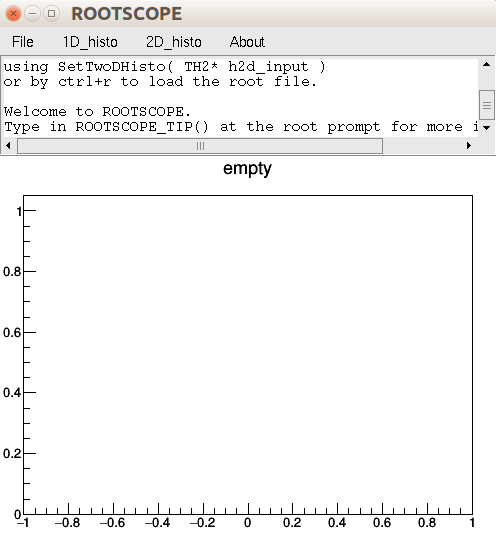
User interface
There are one menu bar, one message box, and a canvas for the display of histograms at the bottom.
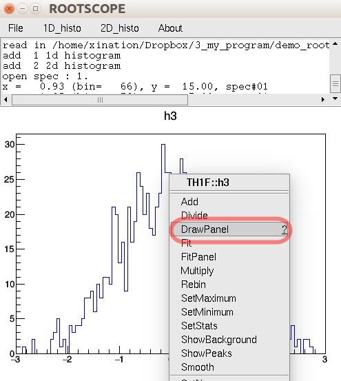
The default ROOT hot keys and right click content menu, etc... are still reserved. For example, right click the histogram will pop up the object-corresponding menu. And you can still use ctrl+s to save to file. One more useful note is that you also can click the histograms, and in the pop-up menu select "DrawPanel".
Operations
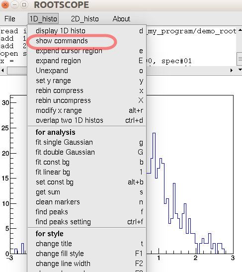
For frequently-used functions, such as Gaussian fit for a peak, there will hot keys for them. For more complicate operation there will be in a dialog form, such as double Gaussian fit. The all hot keys and commands can be found in the drop-down menu. The If you want to change the key binding, it is easy: go to the myROOTSCOPE.C, and search kKey_A (if the original hot key is set to A), and change to whatever you want.
1D Functions
Browsing your histograms
Using mouse to right click the range to expand. Press e key to expand (zoom in). We can use ←/→ arrow or the 4/6 key in the num pad to browse a 1D histogram, and o key to zoom out and restore its original display.
To expand a range more precisely rather than using cursor clicks, one can use E key. or the alt+m key to set an exact cursor position. To clean the markers or other things use n (for no markers).
Switching your histograms
Switching back and forth between your histogram collections can be done by page down and page up keys. To select a histogram or multiple histogram to display, use d key, which standing for displaying 1D histograms. For example, type in "1 2 4" in the entry, then it will display your no.1, no.2, and no.4 histograms. If your input our of the histogram number range, it would not be displayed. Meanwhile, you can display the identical histograms. I.E. "1 1" is valid, in which two panels are the no.1 histogram.
Applying operations your histograms
The d key is very powerful. It allows you to apply operations to your 1D histograms. For example, to add two histograms, overlap two histograms, del one/multiple histograms. Operation is done by typing command in the text entry. The same operation rules are applied to the 2D histograms, which we use A.
PS. In the display dialog, once you finish selecting the histogram(s), you can press "Enter" key or click the "OK" button. Press "Esc" or click the "Cancel" button to cancel the display. ( Currently, the number of histograms to be display in the dialog is 200, but it can store more than 200.)
Operation Rules:
- number is represented to the corresponding 1D histogram.
-
99 = 1 + 2
==> suppose your 1D histograms are fewer than 99, and then 99 represent a new histogram. I.E. we add histogram 1 and 2 to a new histogram, and put it in the end of your histogram list. -
1 = 1 + 2
==> we update our histogram no.1, and the new one will be equal to the original no.1 + no.2. -
1 = -1.5 * 2
==> h1 = -1.5 * h2. Note: the constant's position is fixed at the second number -
99 = 1
==> hnew = h1.(to make a new copy)
-
99 += *
==> hnew = h1 + h2 + h3... (adding up all the histograms)
-
99 += 1..3
==> hnew = h1 + h2 + h3 (use two dots as the range symbol)
-
del 1..3
==> delete h1 h2 h3 (use two dots as the range symbol)
-
del 1 5 2
==> delete h1 h5 h2
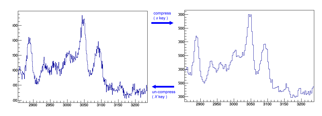
Compress/ un-compress
x key works as to compress the bin, and it is to increase the degree of rebin by 1, which is equal to n=n+1, h->rebin(n). Conversely, X is to decrease the degree of rebin by 1. After rebinning, you can freely go back to its original binning. It is quite handy to check the weak peak that normally requires larger bin size.
Fitting
In a general fitting procedure, we first identify the background level, and then fit the peak. In ROOTSCOPE, it provides two types of background fitting: constant and linear background.
(i) bg = const ==> b key or alt+b
(ii) bg = const + slope * x ==> 1 key
After setting the backgroun,
(i) single Gaussian fit ==> g
(ii) double Gaussian fit ==> G
note: use ctrl + mouse left click to set the two peak centroids.
ROOTSCOPE provides N Gaussian fitting from N = 2 to 10 (by default, N=2)
the above demo clip are for two Gaussian fit .
EX. For 4 Gaussian fit:
(1) press d key to pop-up the 1D histograms list, and then enter: set fitN 4
(2) set background and fitting range.
(3) use ctrl + mouse left click to set the 4 peak centroids.
(4) G, it will pop up initial parameters list (rough estimation), press "ok" button
(5) the results are shown in the top message box.
In generally, linear background setting one can use 1 key, (number 1)
which is to estimate the background by using linear fit for the selected range.
[ALL the data inside the range are used for the fitting]
Alternatively, one can also use l key (small letter l). In this mode,
only the two points that defines the range will be use into the linear fit.
[ONLY TWO points are used]. It provides a rough estimation for the background.
Find peaks
Use f key will add a set of text labels and polymarkers on the screen to indicate the found peaks.
Use ctrl + f to control the threshold and sigma values when searching the peaks or the size of text labels. The threshold is the cutoff value for the peak if its height is less than a certain ratio of the local highest peak, where the default threshold is 10%. The smaller the sigma values are, the more peaks will be identified. Currently, the maximum found peaks are set to 100.
To overlap two 1d histograms
method 1: use d key to open two 1D histograms, then press c key. To toggle c to leave the overlap mode.
method 2: use ctrl + d , then choose two histograms.
To change styles and title
ctrl+t to set title.
F1 is to turn on or off the filling.
F2 is to switch among the 7 different line widths.
F3 is to turn on or off the log scale on the y axis.
2D Functions
Browsing your histograms
For 2D histogram display and operation, we use A key. To set cross-hair markers, we use ctrl+ mouse left click. The hot key setting is very similar to 1D case:
e is to expand a region,
o key is to unzoom,
PgUp and PgDn are to switch 2D histograms
F1, F2, F3, and F4 keys are related to styles.
F1 ==> switch among Draw(), Draw( "col"), Draw("colz").
F2 ==> switch among 4 different marker sizes
F3 ==> switch log scale among x, y, z axis, and none.
F4 ==>switch marker colors.
Gate and projections
The concept of the gate and projection may looks complicated at the first glance. Let's talk about the gate first. A gate is to limit in a certain region. If we gate on y from -1 to 1, then we require the data only comes from y within the this given range. To project to x means that for a given x bin we assign its counts as sum over the gated y bin. i.e. $x_i = \sum_{j_{1}...j_{2}}{C_{ij}}$, where $j_{1}$ and $j_{2}$ are the y gate range.
.
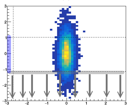
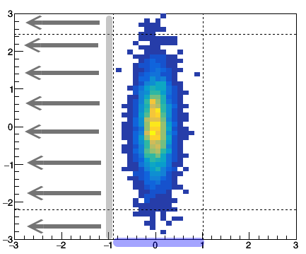
Fig: (left) gating on y [-1 to 1] and then project to x. (right) gating on x [-1 to 1] then project to y.
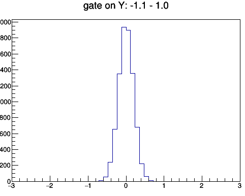
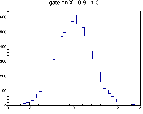
Fig: (left) gating on y [-1 to 1] and then project to x. (right) gating on x [-1 to 1] then project to y.
In real word, we often apply background subtraction, gating, and projection at the same time. In ROOTSCOPE, only constant background is used when doing projection.
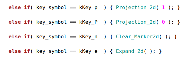
p key for gate on x and project to y.
P key for gate on y and project to x.
For doing projection, we can in the 1D or 2D histogram, since the only needed information is gate range and background value.
In some case, add-and-subtract gating method may be desired.
Use ctrl + p to call the add-and-subtract gating dialog.
2D commands
The majority of the 2D operation is through the command method, i.e. press 'A' key and type in some commands. Please see the full 2D command list.
Here we just illustrated some less intuitive ones.
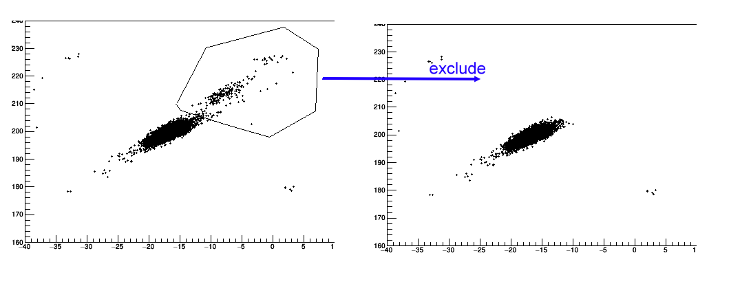
"exclude", it is to exlcude the counts in selected region.
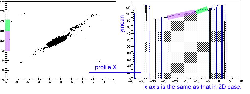
"profile x", it is to create a profile 1D histogram.
It is somewhat similar to TProfile but in TH1 form,
which is useful to examine the relation of y=y(x).
The x axis of the profile histogram will be the same as that in the 2d case,
and the counts is the y mean in a given x bin.
Output and input
ctrl+r to read in all TH1/TH2 objects in a root file.
ctrl+w to write out all TH1/TH2 objects to a root file.
To get the text in the message box widget.
TString ROOTSCOPE::GetMessage()
key table
| For 1D histogram | |
| d | select 1D histograms to display or apply them some operations. |
| mouse right click | set marker (can be used in fit range setting) |
| ctrl + mouse right click | set auxiliary marker ( for double Gaussian fit) |
| alt + m | input the marker position. |
| e | expand into the range set by two markers. |
| shift + e | input a range then zoom into it. |
| o | zoom out. |
| y | set y range |
| alt + r | modify x range (can discard undesired range) |
| pageUp / pageDn | go to previous / next histogram |
| arrow key left / right | move forward / backward of a histogram |
| n | clean out markers etc.. |
| g | single Gaussian fit |
| G | double Gaussian fit |
| b | set const background from two-marker range |
| alt+b | input const background level (for Gaussian fit) |
| 1 | set linear background from two-marker range |
| s | get the sum, bin width, etc... info |
| f | find the peaks |
| ctrl + f | modify the option for peak finding. |
| ctrl + t | modify the title. |
| ctrl + d | choose two histogram to overlap. |
| c | overlap two-displayed histograms |
| x / X | compress / un-compress bin number |
| F1 | change the filling style |
| F2 | change the line width |
| F3 | using log scale in y |
| ctrl + n | add a note to current cursor position |
| ctrl + shift + c | del the current histogram. |
| For 2D histogram | |
| A | select 2D histograms to display or apply them some operations. |
| ctrl + mouse right click | set the marker |
| e | expand into the region set by two markers. |
| shift + e | input a region then zoom into it. |
| o | zoom out. |
| x / X | compress / un-compress the x axis binning |
| y / Y | compress / un-compress the y axis binning |
| z / Z | set min / Max z range |
| pageUp / pageDn | go to previous / next histogram |
| n | clean out markers etc.. |
| s | get the sum, bin width, etc... info |
| ctrl + t | modify the title. |
| p | gating on x and project to y |
| shift + p | gating on y and project to x |
| ctrl + shift + p | get whole range x and y projection. |
| F1 | change the display style ( color or no color) |
| F2 | change marker size |
| F3 | using log scale in x/y/z |
| F4 | change marker color |
commands table
for both 1D and 2D.| 99 = 1+2 | let histo99 = histo1+histo2 |
| 99 = 1.5 * 2 | let histo99 = 1.5 * histo2 |
| 99 = 1.5 * 2 | let histo99 = 1.5 * histo2 |
| 99 += * | let histo99 = sum over all histos |
| del 1 3 5 | del histo 1, 3, and 5 |
| del 1..5 | del histo 1 to 5 |
For 1D: ( press 'd' key, and type in command)
| let x = x+1 | to apply a formula to shift x. (any valid TF1) |
| set fitN 4 | to set N Gaussian fit, N from 2 to 10. |
For 2D: ( press 'A' key, and type in command)
note: the number in [ ] means it is optional,
Ex. the command "sum 2" will work for histogram 2,
"sum" will do the sum operation for the current histogram.
| let x = x+1 | to apply a formula to shift x. (any valid TF1) |
| let y = y+1 | to apply a formula to shift y. (any valid TF1) |
| sum [2] | get the sum over a region at histo2 |
| crop [2] | to keep the data and in a given region while exclude all the rest. |
| exclude [2] | to exclude data in a given region at histo2 |
| exchange axis [2] | to exchange x <==> y axis. |
| overlap 1 2 | to overlap histo1 and histo2 |
| profile x | to create a profile histogram with its counts are the y mean. |
| profile y | to create a profile histogram with its counts are the x mean. |
Contact: