
CoSMo Viewer Program Introduction
CoSMo code is for performing Shell Model calculation developed by Dr. Volya (here is his website about this code). The output of the CosMo code is stored in the xml format. The xml format is well-structured and good for computer to organize smaller scale data. However, it is hard for human to directly use it (not quite intuitive at all for me). So I design a xml parser to extract the essential data, and manipulate the data, such as convert B(E2) or B(M1) to Weisskopf Unit, or to Transition Probability, or combine two xml files, or to view the occupation numbers, etc... You will like it if you need to spend a lot of time to study the CoSMo results.
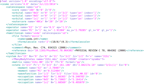
(figure: a demonstration for a xml file)
To run the view_cosmo code
The view_cosmo program is located at '/home/tai/3_programs/cosmo_viewer/' at the polar.physics.fsu.edu server. To run the code, type in ./view_cosmo.py. Its design is to emulate the old-fashion menu-driven program. You type in number to select different functions. To adding xml files to your database, just put the xml files to the cosmo_viewer folder, and the program will automatically parse them.
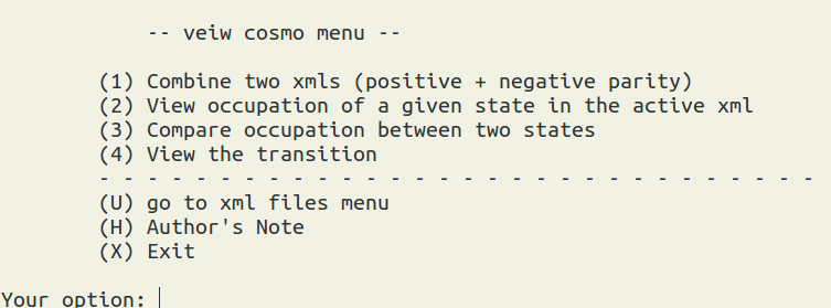
(figure: the menu of view_cosmo program)
Function 1: combine two xml files
In many calculations, we separately calculate the positive and negative parity states. And then we link the two individual xml files together. In CosMo program, it provides Xlevels to concatenate two files. However, the output format is somewhat hard to read for me. In view_cosmo program, type '1', then the program will prompt you to select the two xml files you want to combine.
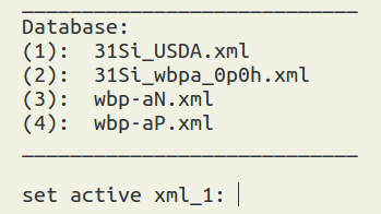
(figure: the xml selection menu)
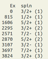
(figure: the output of the combination, Ex = excitation energy in keV, and the numbers in parentheses represent n-th spin. )
Alternative: use level_reader program
Since combine two xml files are frequently use, I specially develop a level_reader program, which is also located at '/home/tai/3_programs/cosmo_viewer/'. To use it. level_reader xml_file1 (xml_file2). This small program can take one or two xml files. The output format is almost identical to the one in view_cosmo. The good things is that you can copy the data from the levels.txt (the output of level reader) to level_factory program directly, to visualize the level scheme. Or use run_cosmo_level.py
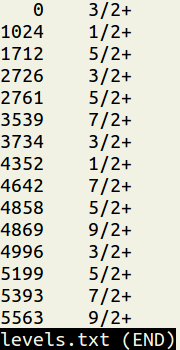
(figure: the output from level_reader)
Function 2: view occupation numbers
To use this function, you have to run the occupation number calculations first (by XSHLAO). Then select the xml file and the state of your interest to view its occupation numbers.
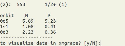
(figure: the output of the occupation numbers. On the top is the state you pick. N = neutron, P = proton.)
You can visualize the occupation numbers as well. It will bring out Xmgrace windows. Sometimes there are some warning messages when open Xmgrace. Just ignore them.
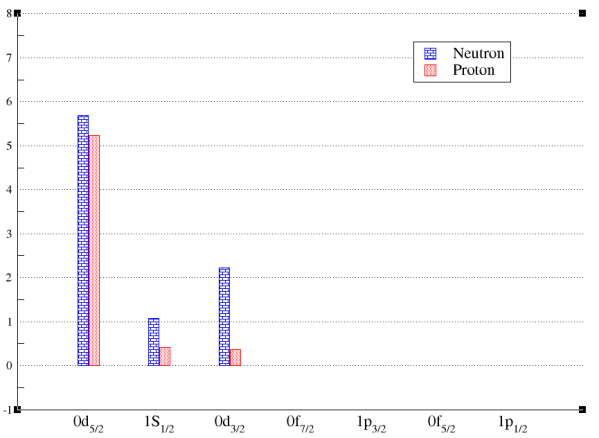
(figure: the bar chart for the occupation numbers of a state.)
Function 3: Compare occupation between two states
To use this function, you have to run the occupation number calculations first (by XSHLAO). Then select the xml file(s) and the two states of your interest to view their relative occupation numbers. Note: the differences of the occupation numbers are calculated from the occupation numbers from the state 1 (the first selection) to substrate the one from the state 2 (the second selection). diff = state1 - state2. You also can visualize the results.
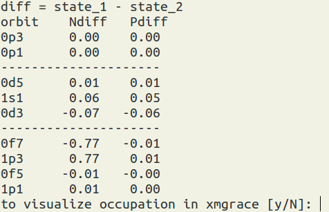
(figure: Ndiff = neutron occupation number difference, P = proton occupation number difference.)
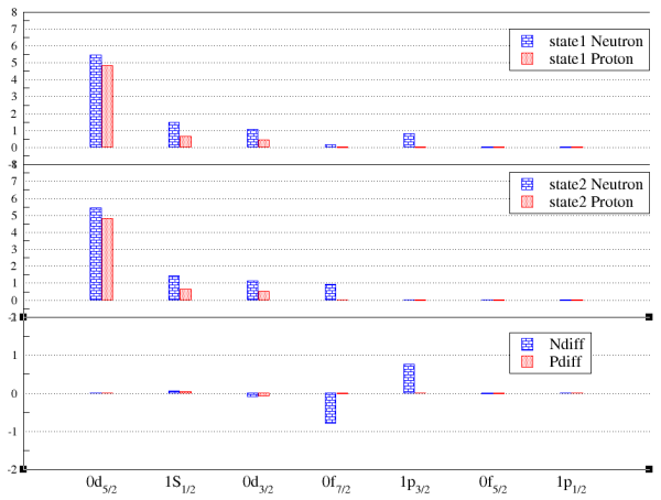
(figure: the bar chart for the occupation number comparison.)
Function 4: View the transition
To use this function, you have to run the occupation number calculations first (by XSHLEMB). Then select the xml file and the state of your interest to view the reduced transition matrix element in the Wessikopf unit or the transition probability in 1/sec. Note: you can use 's' to sort the data. The formula can be seen at here.
![]()
(figure: B(W. U.) = reduced transition matrix element in the Wessikopf unit. trans_Prob = transition probability in 1/sec. The ratio is taken from trans_prob.)
![]()
(figure: the sorting result, it will add up the transitions to the same final state.)
Contact: